Sigmoid和Softmax使用区别（Tensorflow）

一直都对这两个函数的一些概念理不清楚，今天就整理一下，结合吴恩达老师和李沐给出的Tensorflow的coding过程，一并整理厘清概念和这两者的区别。

Sigmoid

Sigmoid通常用于逻辑回归Logistic Regression的二分类中，output出一个概率值（比如：预测一张图片是一只猫的概率）。它的公式为： \[ \frac{1}{1+e^{-z}} \] 图示为:

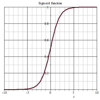
特点：y的值是介于[0,1]之间的，而x是负无穷到正无穷的。x=0时，y=0.5。

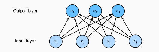
LR的网络结构为:

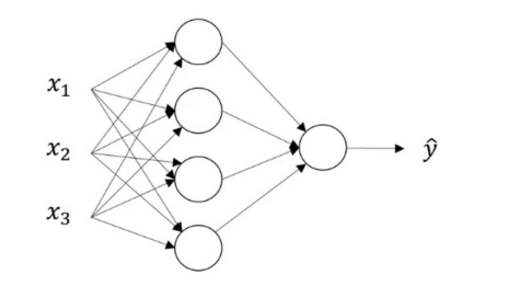
在将Sigmoid用于LR任务中时，模型的输入是一个特征向量X，这时的loss function使用：

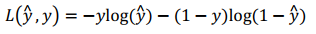
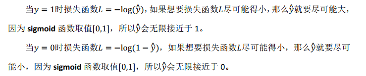
这里不会使用MSE，原因是：

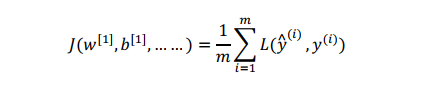
loss function是在单个训练样本中定义的，它衡量的是算法在单个训练样本中表现如何，为了衡量算法在全部训练样本上的表现，需要定义代价函数（cost function），在LR中代价函数即为对m个样本的损失函数求和再平均：

虽然有这么多计算步骤，但是在tensorflow中，我们并不需要自己计算sigmoid后的值a，然后将a和y放到J函数中计算中整体的cost，只需要一个函数就可以帮助我们实现。

tf.nn.sigmoid_cross_entropy_with_logits(logits=z,labels=y)

注意：上述的z是before the final sigmoid activation的值，也就是还没有传入Sigmoid前，只是经过线性计算后的值。

Softmax

softmax函数是对sigmoid的推广，用于处理多分类的问题。公式：

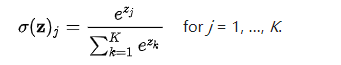
它的输入是一个向量，输出也是一个向量。不同于Sigmoid的输入（实数），输出（介于0,1之间的概率值）。Sigmoid的输出是一个向量，其中 向量中的每一个元素的范围都在(0,1)之间，它能将一个含任意实数的K维向量压缩到另一个K维向量中。

它在线性模型中的应用方式为：对接最后一层，输出一个向量。

它的loss function是:

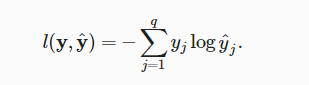
其中q为输出向量y的维度。

那么它的cost function J应该是将整个训练集的损失总和: 通常叫做cross-entropy loss交叉熵损失函数

在tensorflow中该过程只需要一个函数来实现:

tf.reduce_mean(tf.nn.softmax_cross_entropy_with_logits(logits = logits, labels = labels))

• 其中logits也是传入softmax激活函数之前的结果，也就是经过线性计算之后的Z
• logits和labels也必须是相同的shape （num of examples, num_classes）

用tensorflow的完整实现即为:

def compute_cost(Z3, Y):
    """
    Arguments:
    Z3 -- output of forward propagation (output of the last LINEAR unit), of shape (6, number of examples)
    Y -- "true" labels vector placeholder, same shape as Z3
    
    Returns:
    cost - Tensor of the cost function
    """    
    # to fit the tensorflow requirement for tf.nn.softmax_cross_entropy_with_logits(...,...)
    logits = tf.transpose(Z3)
    labels = tf.transpose(Y)  
    cost = tf.reduce_mean(tf.nn.softmax_cross_entropy_with_logits(logits = logits, labels = labels))
    
    return cost

optimizer = tf.train.GradientDescentOptimizer(learning_rate = learning_rate).minimize(cost)
init = tf.global_variables_initializer()
with tf.Session() as sess:
    sess.run(init)
    # Do the training loop
    for epoch in range(num_epochs):

        epoch_cost = 0.                       # Defines a cost related to an epoch
        num_minibatches = int(m / minibatch_size) # number of minibatches of size minibatch_size in the train set
        seed = seed + 1
        minibatches = random_mini_batches(X_train, Y_train, minibatch_size, seed)

        for minibatch in minibatches:

            # Select a minibatch
            (minibatch_X, minibatch_Y) = minibatch

            # IMPORTANT: The line that runs the graph on a minibatch.
            # Run the session to execute the "optimizer" and the "cost", the feedict should contain a minibatch for (X,Y).
            _ , minibatch_cost = sess.run([optimizer, cost], feed_dict={X: minibatch_X, Y: minibatch_Y})

            epoch_cost += minibatch_cost / num_minibatches

            # Print the cost every epoch
            if print_cost == True and epoch % 100 == 0:
                print ("Cost after epoch %i: %f" % (epoch, epoch_cost))
                if print_cost == True and epoch % 5 == 0:
                    costs.append(epoch_cost)    

以上的实现是将里面的计算步骤都展示出来的实现，也就是我们得到Z之后再进一步的得到loss。在李沐的教程中，用tensorflow实现softmax回归使用了更高级的API来实现。

tensorflow keras模块对softmax更简洁的实现

softmax回归的输出层是一个全连接层。因此，为了实现我们的模型，我们只需在Sequential中添加一个带有10个输出的全连接层。同样，在这里，Sequential并不是必要的，但我们可能会形成这种习惯。因为在实现深度模型时，Sequential将无处不在。我们仍然以均值0和标准差0.01随机初始化权重。

net = tf.keras.models.Sequential()
net.add(tf.keras.layers.Flatten(input_shape=(28, 28)))
weight_initializer = tf.keras.initializers.RandomNormal(mean=0.0, stddev=0.01)
net.add(tf.keras.layers.Dense(10, kernel_initializer=weight_initializer))

以上实现的输入是28*28大小的灰度图片，分类类别数为10。

在这里，我们使用学习率为0.1的小批量随机梯度下降作为优化算法

loss = tf.keras.losses.SparseCategoricalCrossentropy(from_logits=True)
trainer = tf.keras.optimizers.SGD(learning_rate=.1)
num_epochs = 10
d2l.train_ch3(net, train_iter, test_iter, loss, num_epochs, trainer)