Attention and Transformer model
斯坦福cs231n最新的课程中包含了attention的模型讲解,但是很可惜我们现在只能看到17年的老课程,在youtube上可以找到,课程主页是cs231n。可以在课程主页中下载对应的slides和查看推荐的blog,都是学习attention机制的好教材。另外我在学习cs231n课程过程中,也参考了吴恩达对于sequence model的讲解,它课程中也涉及到了attention机制,课后作业也包含了简单的attention机制的实现,可以作为辅助理解来看。这篇博客权当自己学习attention以及由此创造的attention系列模型比如transformer的记录。cs231n推荐的博客内容也是很通俗易懂,英文不好的同学有中文翻译可以参考。
general attention model
RNN有多种类型的网络:
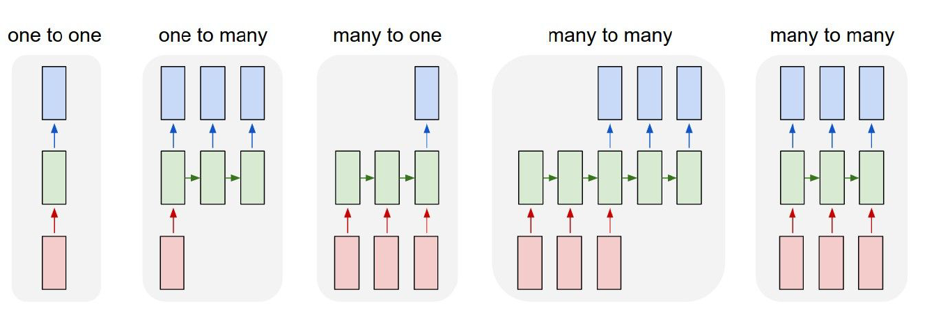
对于"many to many"类型的网络,有可能输入的长度不等于输出的长度,在机器翻译的任务中很常见。这种网络也叫Sequence to Sequence,首先该网络会经由encoder对输入进行编码,然后再有decoder进行sequence的生成。但是这种网络在长句子中表现很差,如果输入句子的长度很长,encoder网络就很难记忆住所有信息,从而在decoder中翻译出准确的词语。由此,需要用到attention model。从计算角度来说就是encoder每次都会产生一个固定长度的vector,这对于长句子来说fixed length的向量很难记住很早之前的信息:
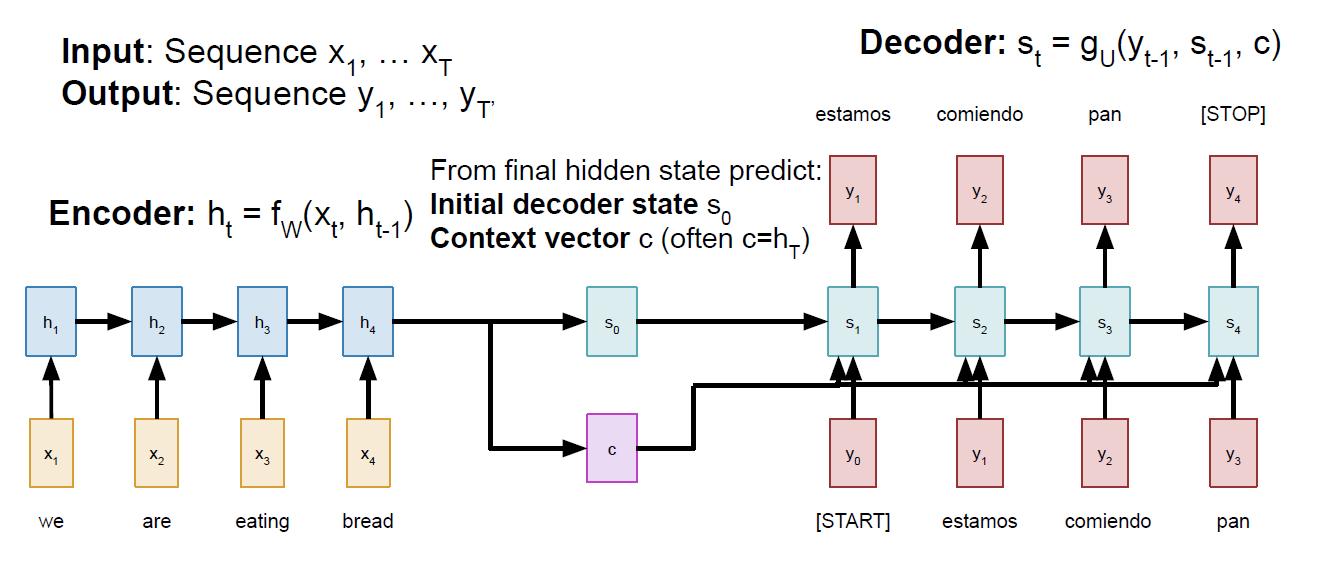
那为了解决一个fixed length的vector很难记忆前序信息的缺陷,所以诞生了attention 机制!具体的就是在decoder阶段的每一个时间步利用都产生不同的context,这个context产生的过程就是attention计算的过程。主要思想是在产生y之前做一个attention的权重计算,这个权重指的是在计算某个时间步的y值时,我们应该对输入句子的每一个词给予多少关注,给予的关注多,权重就大。所以这里我们会基于initial decoder state(previous hidden state of the (post-attention) LSTM)和encoder网络的输出值计算权重,计算过程采用dense layer.这些权重值的和是1。
对于很长输入的句子,encoder不再是输出一个固定的context。如下:
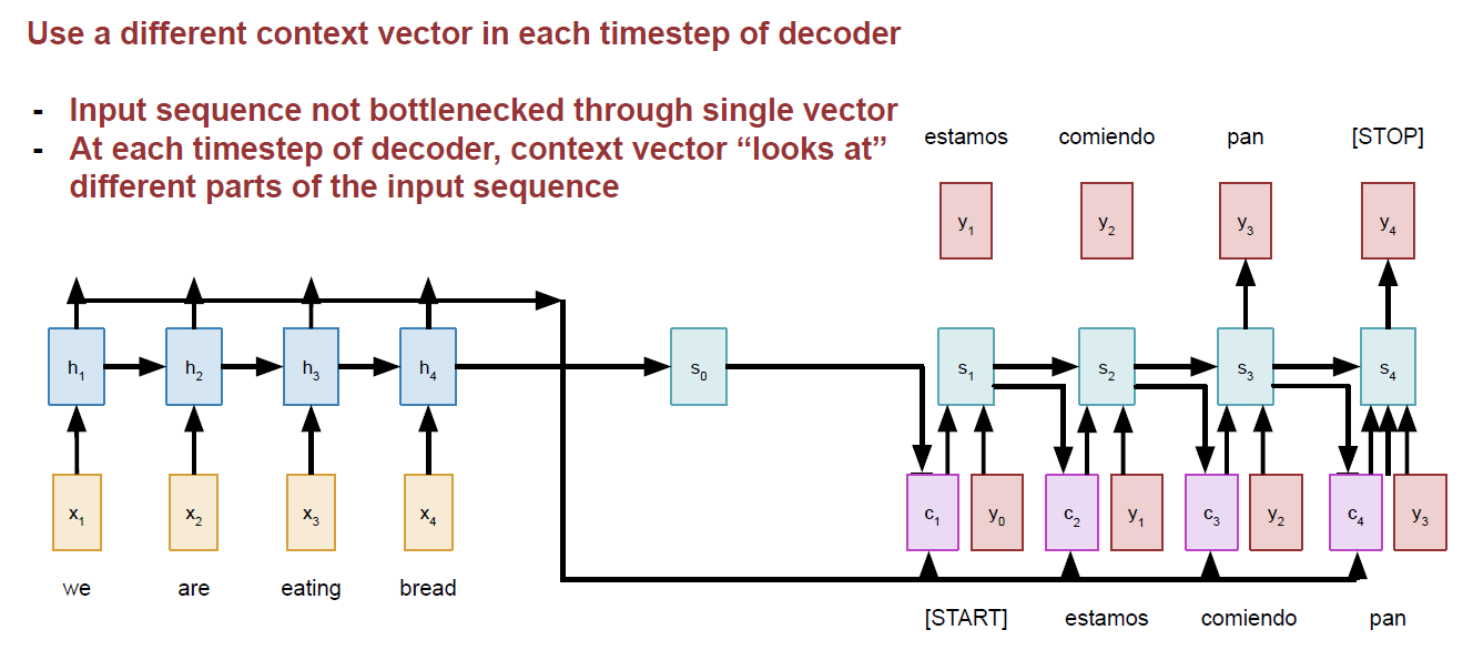
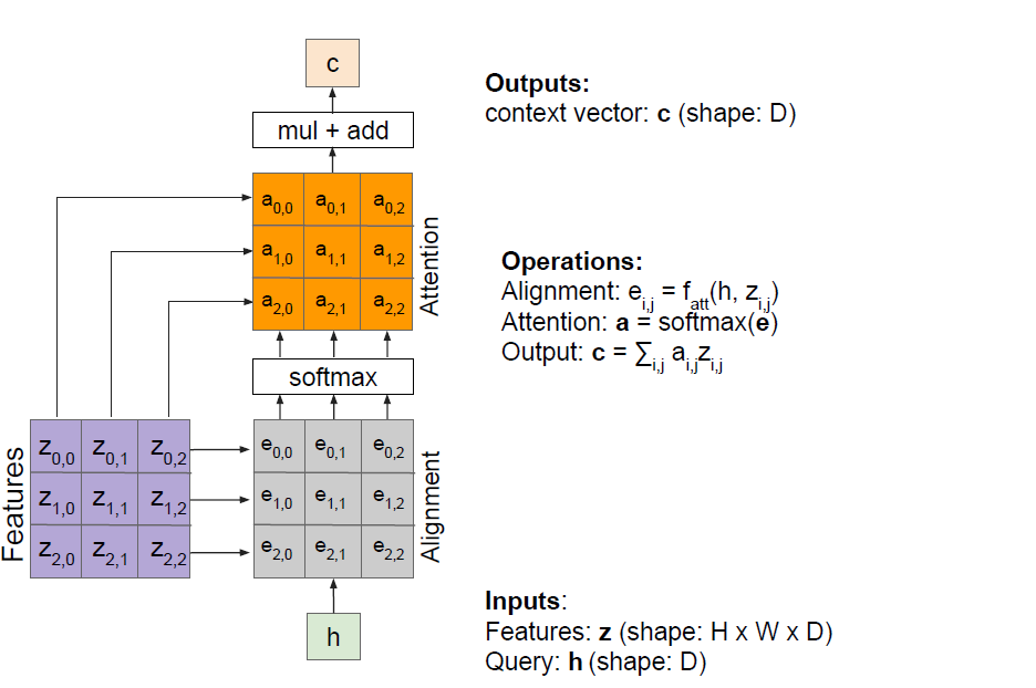
context的详细计算如下:
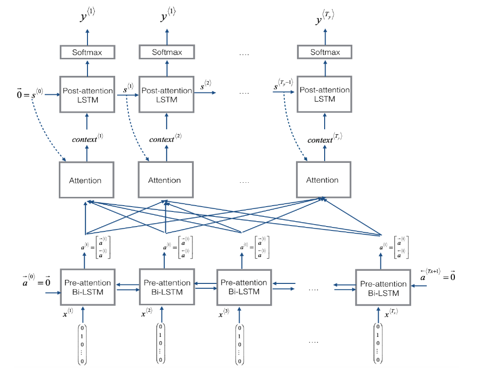
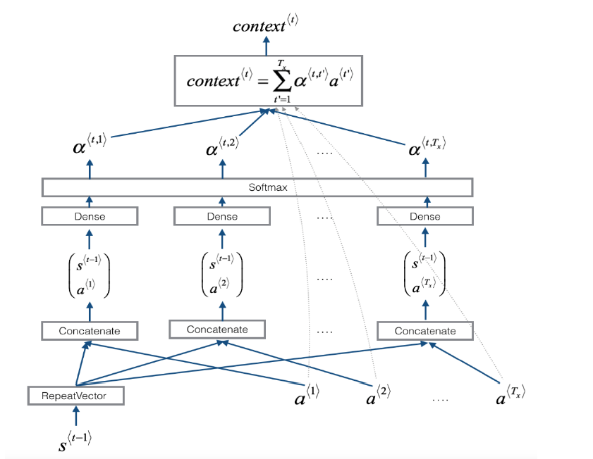
上面两张图是吴恩达在深度学习专项课程中的讲解细节,在cs231n的图中可以看出来它将dense
layer的输出单独列出来了,也就是下图中alignment
scores(e),在e的基础上再计算attention
weights(a),所有的attention weights总和为1 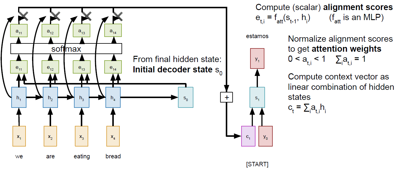
但是总体来说两个的讲解方式是一致的,cs231n这门课为什么把其中的e单独拎出来也是有它的用意,主要为了后面讲解self-attention。这里我琢磨了好一会儿才明白。还有一点值得提一下,吴恩达的图里那个与hidden
state 一同输入进dense
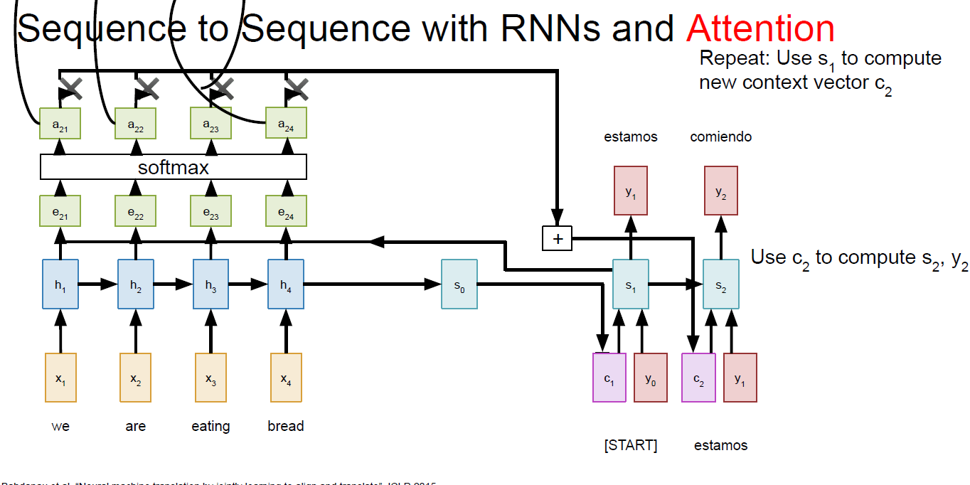
layer的repeateVector不要搞混淆,其实这里每次在decoder的一个时间步计算context时用到的s都不一样,比如在上面的里,计算c1用的是encoder的最后一个hidden
state,而计算C2的时候我们需要用decoder的第一个时间步的hidden
state来计算:
这种attention计算机制如果用到image caption上面如何做呢?获取图片的特征我们使用CNN来抓取,得到的feature map用来当作rnn中的hidden state计算:
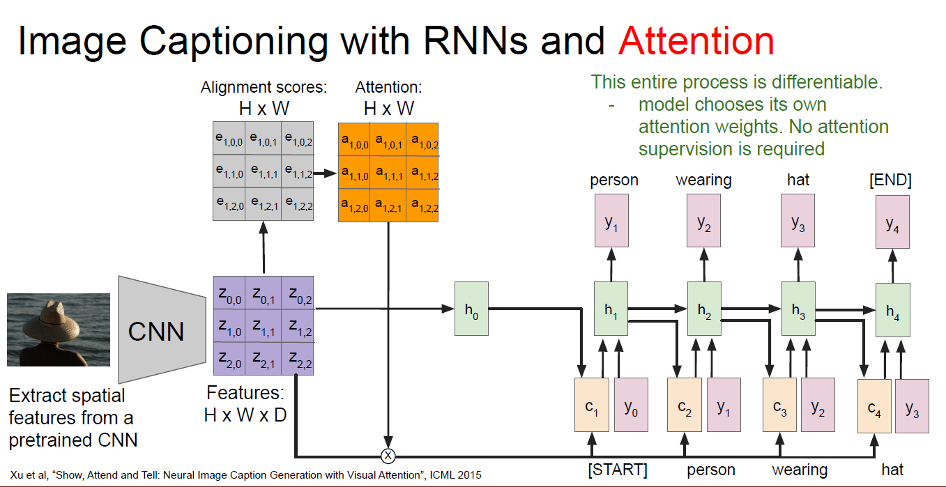
理解以上的原理很重要,再把上面这个图改写一下,将h变成decoder的query:
以上都是简单的attention机制,随后的transformer模型真正的将attention机制推广开来,见transformer的paper
Attention is all you need 2017
在transformer的paper中,作者首先介绍本文:主流的sequence tranduction模型主要基于复杂的RNN或者CNN模型,它们包含encoder和decoder两部分,其中表现最好的模型在encoder和decoder之间增加了attention mechanism。本文提出了一个新的简单的网络结构名叫transformer,也是完全基于attention机制,"dispensing with recurrence and convolutions entirely"! 根本无需循环和卷积!了不起的Network~
在阅读这篇文章之前需要提前了解我在另外一篇博客 Attention and transformer model中的知识,在translation领域我们的科学家们是如何从RNN循环神经网络过渡到CNN,然后最终是transformer的天下的状态。技术经过了一轮轮的迭代,每一种基础模型架构提出后,会不断的有文章提出新的改进,文章千千万,不可能全部读完,就精读一些经典文章就好,Vaswani这篇文章是NMT领域必读paper,文章不长,加上参考文献才12页,介绍部分非常简单,导致这篇文章的入门门槛很高(个人感觉)。我一开始先读的这篇文章,发现啃不下去,又去找了很多资料来看,其中对我非常帮助的有很多:
- 非常通俗易懂的blog 有中文版本的翻译
- Neural Machine Translation: A Review and Survey 虽然这篇paper很长,90+页。前六章可以作为参照,不多25页左右,写的非常好
- stanford cs231n课程的ppt 斯坦福这个课程真的很棒,youtube上可以找到17年的视频,17年的课程中没有attention的内容,所以就姑且看看ppt吧,希望斯坦福有朝一日能将最新的课程分享出来,也算是做贡献了
- cs231n推荐的阅读博客 非常全面的整理,强烈建议食用. 这位作者也附上了自己的transformer实现,在它参考的那些github实现里,哈佛大学的pytorch实现也值得借鉴。
Transformer这篇文章有几个主要的创新点:
- 使用self-attention机制,并首次提出使用multi-head attention
该机制作用是在编码当前word的时候,这个self-attention就会告诉我们编码这个词语我们应该放多少注意力在这个句子中其他的词语身上,说白了其实就是计算当前词语和其他词语的关系。这也是CNN用于解决NMT问题时用不同width的kernel来扫input metric的原因。
multi-head的意思是我使用多个不同的self-attention layer来处理我们的输入,直观感觉是训练的参数更多了,模型的表现力自然要好一点。
- Positional embeddings
前一个创新点解决了dependence的问题,那如何解决位置的问题呢?也就是我这个词在编码的时候或者解码的时候应该放置在句子的哪个位置上。文章就用pisitional embedding来解决这个问题。这个positional embedding和input embedding拥有相同的shape,所以两者可以直接相加。transformer这篇文章提供了两种encoding方式:
1) sunusoidal positional encoding
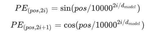
其中,pos=1,...,L(L是input句子的长度),i是某一个PE中的一个维度,取值范围是1到dmodel。python实现为:
1 | def positional_encoding(length, depth): |
2) learned positional encoding
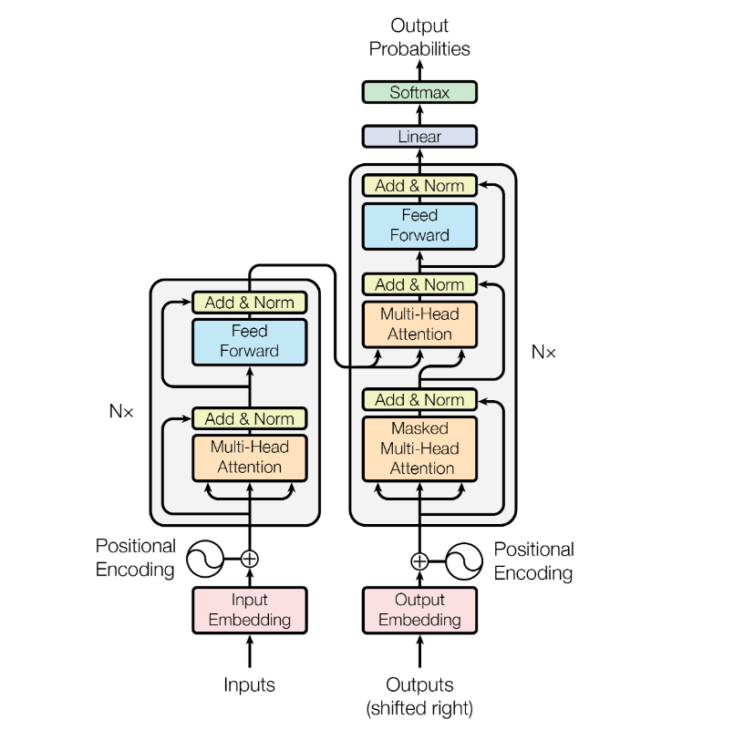
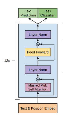
整体上看,这篇文章提出的transformer模型在做translation的任务时,架构是这样的:
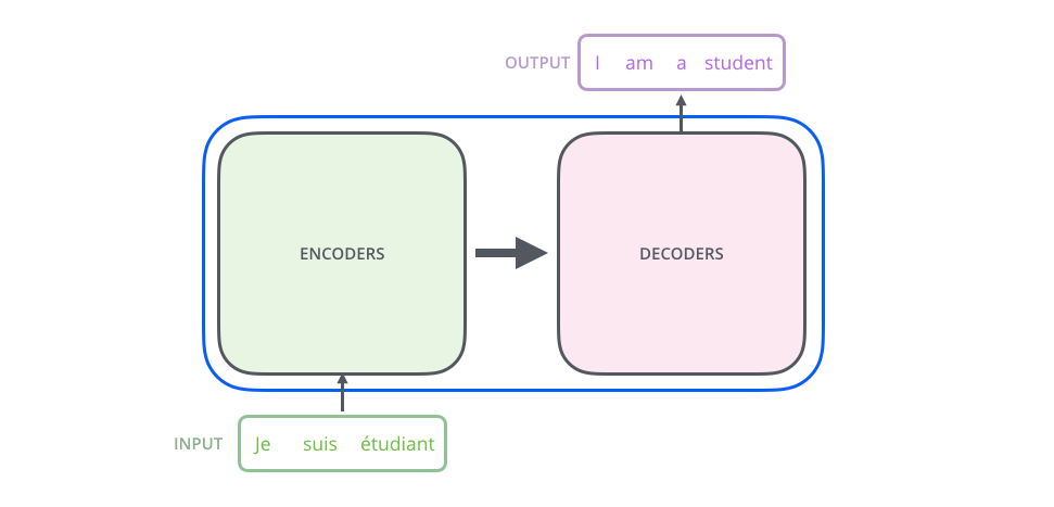
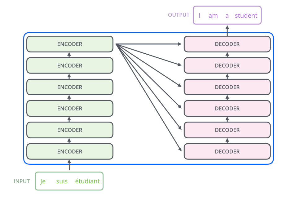
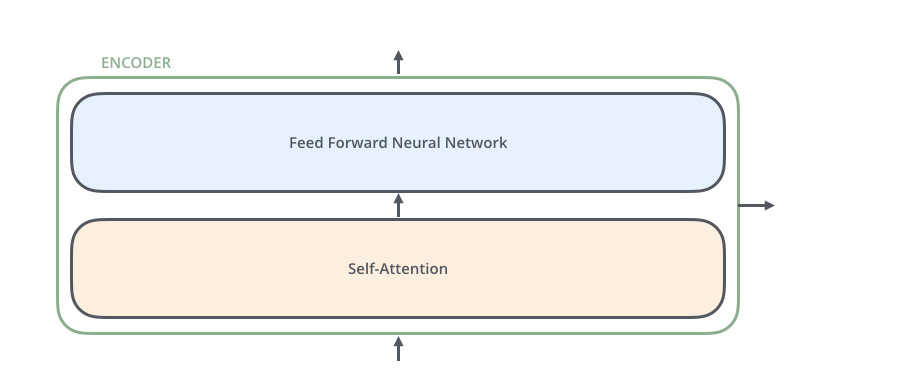
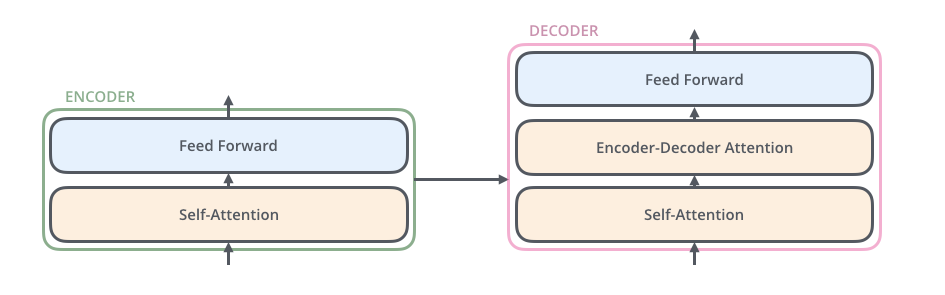
其中encoders部分包含了6个encoders的block,decoders部分也包含了6个decoders的block,将encoders的每一个block拆开来看,有两个sub layer:
其中decoder部分的block比encoder部分的block多了一个sub layer,其中self-attention和encoder-decoder attention都是multi-head attention layer,只不过decoder部分的第一个multi-head attention layer是一个masked multi-head attention,为了防止未来的信息泄露给当下(prevent positions from attending to the future).
在transformer模型中,作者还使用了residual connection,所以在encoder的每一个block中,数据的flow是:
其中self-attention中涉及的运算details是:
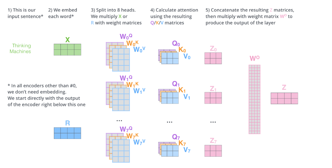
可以发现其中涉及的运算都是矩阵的点乘,并没有RNN中那种时间步的概念,所以所有运算都是可以parallelizable,这就能使得模型的推理和训练更加的efficient。并且!Transformers也可以抓住distant的依赖,而不是像rnn那样对于长依赖并不是很擅长,因为它前面的信息如果像传递到很后面的单词推理上,需要经历很多时间步的计算,而transformer在推理每一个单词的时候都可以access到input句子中的每一个单词(毕竟我们的Z中包含了每一个单词跟其他单词的关系)。
其中positional encoding现在可以简单的理解成在我们编码的word embedding上我们又加了一个positional encoding,维度和我们的embedding一模一样。
在tensorflow中有一个layer是
MultiHeadAttention,如果我们想实现transformer里的这个self-attention,那就是query,key,value其实都是由input vector计算来的。
以上的理论计算看起来可能会有点模糊,可以同步参照博客 参考 illustrated transformer介绍的详细细节,基于tensorflow框架实现的transformer来帮助自己理解transformer模型。
encoder部分
encoder的每一个block由两个sub-layer组成,中间穿插resnet connection。
![]()
1 | def multihead_attention(self, query, memory=None, mask=None, scope='attn'): |
decoder部分
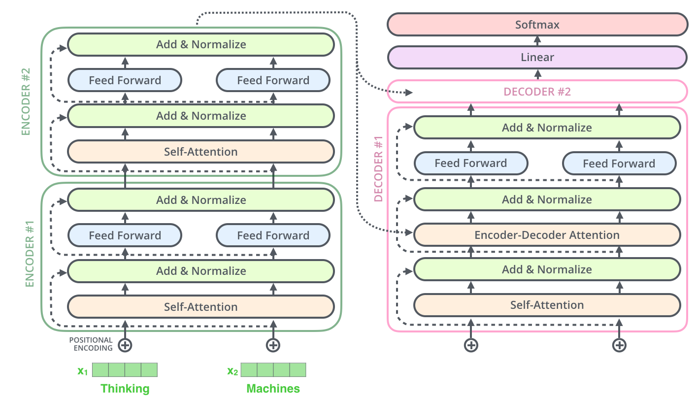
在decoder部分,我们可以看到每一个decoder block的输入有两个:整个encoder部分的输出以及上一个decoder block的输出(第一个decoder block是词向量的输入),而encoder部分的输出是接到每一个decoder block的第二个sublayer的。正如刚刚提到了,decoder部分的每一个block跟encoder部分的block有一个不一样的地方,那就是多了一个sublayer: encoder-decoder attention。至于encoder部分和decoder部分是如何connect的,
The encoder start by processing the input sequence. The output of the top encoder is then transformed into a set of attention vectors K and V. These are to be used by each decoder in its “encoder-decoder attention” layer which helps the decoder focus on appropriate places in the input sequence
也就是我们得到了encoder部分top layer(最后一个encoder
layer)的输出之后,我们将输出转化成K和V.
我们可以看到在multihead_attention里,memory是enc_out
1 | def decoder_layer(self, target, enc_out, input_mask, target_mask, scope): |
以上实现的transformer其实我觉得还是有一点点复杂,毕竟在tensorflow2.0+版本中已经有了官方实现好的layers.MultiHeadAttention可以使用,应该可以大大简化我们实现步骤,特别是上面的def multihead_attention(self, query, memory=None, mask=None, scope='attn'):。从刚刚的实现里我们可以发现,除了decoder部分每一个block的第二个sublayer的attention计算有一点不一样之外,其他的attention计算都是一模一样的。我在github上找了不少用TF2.0实现的transformer(最标准的也是Attention
is all you
need的模型),发现很多都都写得一般般,最终发现还是tensorflow官方文档写的tutotial写的最好.
现在对照tensorflow的tutorial以及上面transformer的计算过程,拆解一下官方给的代码。
首先定义一个baseAttention类,然后在此基础上我们再定义encoder和decoder中的attention:
1 | class BaseAttention(tf.keras.layers.Layer): |
那么针对encoder结果输入到decoder的cross attention layer怎么处理呢?这时候我们使用MultiHeadAttention时就需要将target sequence x当作是query,将encoder输出当作是context sequence也就是key/value。
1 | class CrossAttention(BaseAttention): # encoder结果输入到decoder的层 |
然后我们再定义global attention,global attention就是没有任何特殊操作的(比如上面的attention计算它有特别的context),而在transformor中更多的是self-attention,也就是我们传递给MultiHeadAttention的query,key,value都是同一个值。
1 | class GlobalSelfAttention(BaseAttention): |
最后我们定义causal self attention layer,这个是在decoder的每一个block的第一个sublayer:self-attention layer.其实这个layer是和global attention layer差不多的,但还是有一点微小的差别。为什么呢?因为我们在decoder阶段,我们是一个词语一个词语的预测的,这其实包含了一层因果关系,我们在预测一个词语的时候,我们应该已知它前面一个词语是什么,RNN中的hidden state传递到下一个时间步就是这个因果关系的传递。那么如果我们使用刚刚我们实现的global attention layer来实现这个self attention,并没有包含这个因果关系,不仅如此,如果我们使用常规的self attention的计算,将target sequence全部当作输入输入到decoder中的第一个block中,会有未来的数据提前被当前时刻看到的风险,所以在Transformer这篇文章中,作者提出使用mask的技术来避免这个问题。
在tensorflow中实现很简单,就只需要给MultiHeadAttention传递一个use_causal_mask = True的参数即可:
1 | class CausalSelfAttention(BaseAttention): |
这样就可以保证先前的sequence并不依赖于之后的elements。这里我本来有一个疑问是,这样一来这个causal layer并不能实现bi-rnn的能力?但后来一想并不是,因为双向的RNN的后向是指后面的词语先输入,其实就是从后往前输入,这样就可以知道一个sequence当前词语依赖于后面的词语的权重。
why transformer?
这里想补充一个东西,在从encoder-decoder过渡到transformer的时候,我一直的疑问是为什么要用transformer呢?为什么Effective Approaches to Attention-based Neural Machine Translation这篇paper介绍的方法就渐渐不被人所用了呢?一开始我去看了下transformer的原文,发现paper介绍的非常简单,所以就去找了下博客,找到一篇解释为什么transformer比LSTM快的博客
文章说在传统的也就是paper:Neural Machine Translation by Jointly Learning to Align and Translate中介绍的用LSTM的encoder-decoder架构来做机器翻译的问题,一个问题在于:在RNN模型中,我们在计算当前时间步时,需要使用到前一个时间步的hidden_state,这就造成一个问题是无法并行训练,你必须要等到前面的东西都输完了你才能计算当前时间步的结果。transformer就可以解决这个问题,它完全摒弃了RNN的结构,基本上是一个FCNN。首先我们都知道输入到模型中来的是一个序列,序列中的每一个单词我们都转化为了词向量。如果是传统的RNN模型,这时候就要一个vector一个vector的往RNN里输入了,但transformer不是,它是将这个embedding变幻成了三个向量空间,也就是我们后面看到的Q,K,V.
后面又去谷歌了一番,找到一个stack上的问题,也有人有这个疑问,被采取的回答总结起来就是:
- transformer避免了recursion,从而可以方便并行运算(减少了训练时间),这个说法其实跟上面博客一个意思
- 同时transformer在长句子的dependency上提高了performance
- Non sequential: sentences are processed as a whole rather than word by word.
- Self Attention: this is the newly introduced 'unit' used to compute similarity scores between words in a sentence.
- Positional embeddings: another innovation introduced to replace recurrence. The idea is to use fixed or learned weights which encode information related to a specific position of a token in a sentence.
transformer并没有long dependency的问题,为什么?我们知道transformer的做法是将整个sequence作为一个整体输入到模型。也就是它在预测当前时间步的word时并不依赖于上一个时间步的状态,模型看到的是整个序列,也许有人会质疑双向RNN不是也可以解决这个问题吗,但是这个作者说双向RNN仍然不能彻底解决长句子的依赖问题。
其实在机器翻译领域,为了解决长句子的依赖问题,CNN曾经也被广泛用于解决这个问题,不仅如此,CNN还有共享参数的优点,也就是可以在GPU上并行计算。如何用CNN处理句子可以参考paper,CNN解决依赖问题是用不同宽度的kernel去学习依赖,比如width=2就学习两个词之间的依赖关系,width=3就学习三个词之间的依赖,但长句子的依赖很可能会有很多组合,所以就需要使用到很多不同宽度的kernel,这是不现实的。虽然现在CNN不怎么用来解决S2S的问题,但我觉得它是RNN结构的模型过度到transformer的一个中间桥梁,同时也可以帮助我们理解attention is all your need这篇文章。感兴趣的可以读一下Convolutional Sequence to Sequence Learning 2017
drawbacks and variants of transformer
transformer的一个很大的问题是它的计算量是随着sequence长度的增加而指数型增加的,从矩阵运算我们就可以发现每一个单词都和句子中的其他单词做了attention score的计算。所以自从17年transformer模型出来之后,很多用于改进transformer计算效率的小改动paper出了不少,详见Do Transformer Modifications Transfer Across Implementations and Applications?. 但这篇文章的作者发现:
Surprisingly, we find that most modifications do not meaningfully improve performance.
也就是说这些文章的改动更多的依赖于实现细节,并没有对tansformer的性能有本质上的提高。
另外,对于positional encoding也有不少researcher做了功课,比如relative linear postion attention,dependency syntax-based position等。
tensorflow API实现补充介绍
tf.keras.layers.MultiHeadAttention
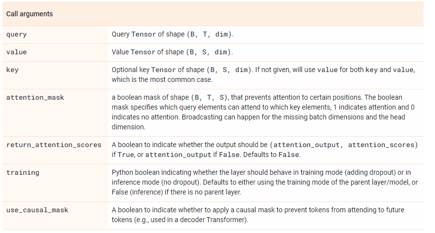
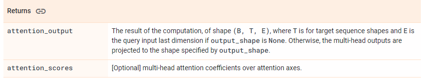
注意,return的结果包含两个,其中attention_output的shape的第二维是和target sequence的长度是一致的,并且E是和query的最后一维是一致的。
https://dl.acm.org/doi/10.5555/3305381.3305510)
Attention Family
这个章节整理于blog,这个作者之前写了一篇介绍attention的文章,后面在2023年一月的时候又更新了两篇博客,详细介绍了从2020年以来出现的新的Transformer models。权当自己学习记录一些我还需要补充的知识。
The Transformer (which will be referred to as “vanilla Transformer” to distinguish it from other enhanced versions; Vaswani, et al., 2017) model has an encoder-decoder architecture, as commonly used in many NMT models. Later simplified Transformer was shown to achieve great performance in language modeling tasks, like in encoder-only BERT or decoder-only GPT.
pretraining
pretraining的技术在NLP领域取得了空前的发展,比如我们熟知的GPT系列模型以及Bert模型。自从transformer应运而生之后,pretrain的技术就发展开来。
model pretrain的方式有三种:decoders,encoders,encoder-decoders:
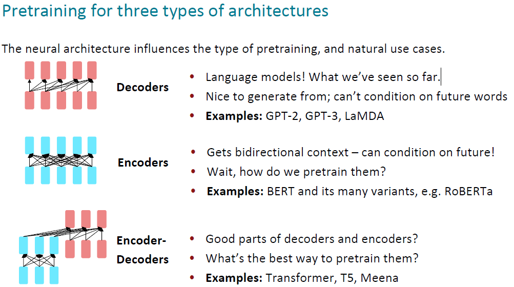
上图中第一个将transformer中decoders拿来做pre-train的模型是GPT,paper是:Improving Language Understanding by Generative Pre-Training
GPT模型分为两个阶段,第一个阶段是unsupervised learning,第二个是supervised learning。首先第一阶段是一个典型的language modeling模型,目标函数是:
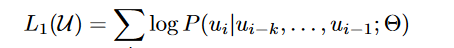
其中k是context窗口的大小,也就是我们预测一个单词的时候,只看它前k个单词,在前k个单词的基础上使得出现当前单词的概率最大。至于这个模型是什么?其实就是我们熟知的transformer decoder部分,包含multi-head self-attention(注意这里是masked的attention,原因我们只看前k个单词,并不看后面的部分)和feed-forward:
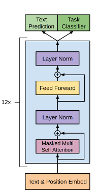
我们取最上层的decoder的输出,然后使用softmax来预测p(u)。以上的decoder模型在一个很大的语料库上进行训练之后,我们预训练部分就做完了,通过这一步我们拥有了一个decoder,它的作用是当我们每次输入一个sentence,它会告诉我们紧接着的那个单词是什么。
接着第二部分是我们的监督学习,原文说监督学习部分需要在不同的task上进行fine-tune:
First, we use a language modeling objective on the unlabeled data to learn the initial parameters of a neural network model. Subsequently, we adapt these parameters to a target task using the corresponding supervised objective.
第二种用于pre-train的模型架构是encoders。它和用decoder来做非监督学习不一样的地方在于,摘录自博客OpenAI GPT: Generative Pre-Training for Language Understanding
Open AI GPT uses a Transformer Decoder architecture as opposed to BERT’s Transformer Encoder architecture. I have already covered the difference between the Transformer Encoder and Decoder in this post; however, it is as follows:
- The Transformer Encoder is essentially a Bidirectional Self-Attentive Model, that uses all the tokens in a sequence to attend each token in that sequence
i.e. for a given word, the attention is computed using all the words in the sentence and not just the words preceding the given word in one of the left-to-right or right-to-left traversal order.
- While the Transformer Decoder, is a Unidirectional Self-Attentive Model, that uses only the tokens preceding a given token in the sequence to attend that token
i.e. for a given word, the attention is computed using only the words preceding the given word in that sentence according to the traversal order, left-to-right or right-to-left.
— from BERT: Pre-Training of Transformers for Language Understanding
Thus, GPT gets its auto-regressive nature from this directionality provided by the Transformer Decoder as it uses just the previous tokens from the sequence to predict the next token.
在这里典型的代表就是Bert.
参考读物:
- OpenAI GPT: Generative Pre-Training for Language Understanding
- Bert's Transformer Encoder architecture
Bert:Pre-training of Deep Bidirectional Transformers for Language Understanding 2019
这篇文章出现在openai的GPT模型之前,前身是ELMo。
有两种方式将pre-trained language representations用于下游任务,第一种是feature-based,第二种是fine-tine,其中第一种代表是ELMo,将pre-trained representations用于附加的features输入到下游任务中;第二种是得到pre-trained的representation之后,将模型接入下游任务,然后同时fine-tune所有的参数。
作者在finetune模型时,采取11个下游任务:
- GLUE general language understanding evalation
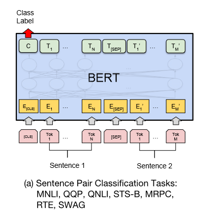
它的输入主要是sentence pair。比如MNLI数据集就是区分输入的两个句子,后者跟前者是entailment,contradiction还是中立的关系。另外GLUE benchmark中还包含其他的几个数据集:QQP(比较两个question是不是语义上近似的),QNLI(问答数据集,sentence中是否包含能够回答question的answer)等。
Bert在处理此类任务的时候,不是单独对两个句子分别编码的,而是将两个句子拼接在一起,共同输入给self-attention,并且在两个句子中间加了一个标志[SEP]。在fine-tune的时候,直接将输出的hidden states的中的第一个token的向量输出到全连接层中接softmax分类器。
- SQuAD v1.1 stanford question answering dataset
数据集的结构是一个question,一个passage,这个passage里面包含answer。该任务是预测answer在passage中的哪儿。在fine-tune的过程中引入了start和end两个vector,毕竟我们想知道这个answer在passage的哪个位置:
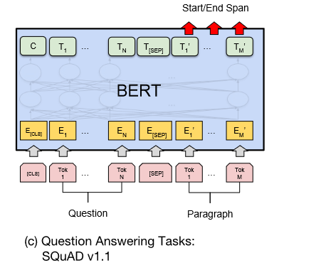
这里做分类的时候不是用的全连接层,而是使用的dot product:
其中,S是start vector,i是指位置i的token word,Pi指位置i的word成为start的概率。
作者还在SQuAD v2.0上做了实验,这个数据集和1.1不一样的地方在于数据集中包含不存在answer的情况。
- SWAG situation with adversatial generations
在阅读本篇文章的过程中一个有一个疑问就是,其实bert的思想并不陌生,有点像之前的word2vec,那为什么现在大家不用预训练的word2vec来解决问题了呢?在Bert原文的第二章节,作者解答了这个问题:
The advantage of these approaches is that few parameters need to be learned from scratch.
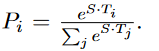
同样在cs224n的课件上我们也可以看到为什么大家转而从静态的词向量投向了GPT,Bert:
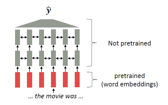
上面这张图说明的是以往的用预训练的词向量用于模型的方式,可以看到大多数的模型参数是随机初始化的,只是模型的输入部分是我们预训练的词向量。
但是在model nlp内,我们可以看到所有的参数在初始化的时候都是使用的预训练好的参数。这一类模型可以在预训练的过程中学习到如何表示一整个句子。
Improving Language Understanding by Generative Pre-Training 2018
GPT stands for "Generative pretrained transformer" or "generative pre-trained"
two main reasons for leveraging more than word-level information from unlabeled text data
- unclear about what type of optimization objectives are most effective at learning text representations that are useful for transfer 缺乏很好的优化函数
- Second, there is no consensus on the most effective way to transfer these learned representations to the target task 如何更有效的将pre-train的知识transfer到target task还没有很好的方法
作者在introduction部分强调了自己提出的模型在fine-tune阶段只需要对模型架构进行微调便可以适应target task,在知识迁移时,采用了paper: Reasoning about entailment with neural attention,which process structured text input as a single contiguous sequence of tokens.
Related work : LSTM using as the pre-trained network to capture the representation but they has lots of restrictions. This paper use transformer networks to allow capturing longer range linguistic structure. Further, in fine-tuning process, the model only requires minimal changes to model architecture other than involving substantial amount of new parameters.
Framework
1. unsupervised pre-train process
以当前token的前k个单词为context,预测当前token。典型的language modeling。
2. Supervised fine-tuning
这里和Bert不一样的是,作者采用了两个目标,第一个目标是target task的目标(比如分类),第二个目标是pre-train时候的language modeling的目标,即预测当前词语。为什么这么设定?作者的意思是将language modeling的目标加入模型的fine-tune阶段可以增加模型的泛化能力和加速收敛。所以整体的模型架构是:
截至到目前,如果我们的下游任务是分类任务,模型的fine-tune是很简单的,就将decoder的输出的最后一个token的vector拿出来接一个classifier就可以了,但是如果处理QA,texttual entailment的数据集任务,这一类的任务的输入往往是句子的pair或者question,answer的组合。这时候作者想到一个办法是,将他们都当成一个连续的sequence,并在其中增加了随机初始化的vectors比如start/END. 同时作者指出之前有一些论文在这个方面也做了不少research,但都是“re-introduce a significant amount of task-specific customization and does not use transfer learning for these additional architectural components”. 那么具体是如何对模型的输入进行小改造的,如图:
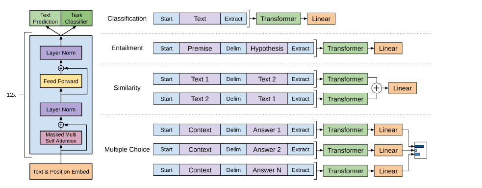
其中对于QA的task,作者的处理有一丢丢特殊,我们拿到的数据是一系列context,question和一系列answers,作者将document context,question和answer拼接在一起变成一整个sequence输入到decoder中,然后计算当前question和answer的匹配程度。
Experiment
dataset : BooksCorpus dataset contains 7000 unique books
Analysis
- 随着decoder部分层数的增加,performance会越来越好。作者得出结论 ”This indicates that each layer in the pre-trained model contains useful functionality for solving target tasks“
- zero-shot
- ablation studies 作者在fine-tune阶段将LM任务去除,其实这时候和Bert finetune阶段是一模一样的,只有target task的任务需要优化。作者从这个实验中得出的结论是:LM可以在NLI和QQP两个任务上帮助提高performance。同时也发现,更大的数据集会从LM任务中获利更多,但小数据集并不会获利。同时作者将模型不进行pretrain,直接在数据集上训练,发现如果没有pretrain,所有的任务的performance都会下降,以此证明pre-train确实给所有任务都带来了performance的提升
Conclusions
GPT的两个关键词: generative pre-training & discriminative fine-tuning
同时作者得出结论是:在Transformer(what models)上利用text with long range dependencies(which dataset to use)会收获好的performance。
本文推荐阅读材料
Reference
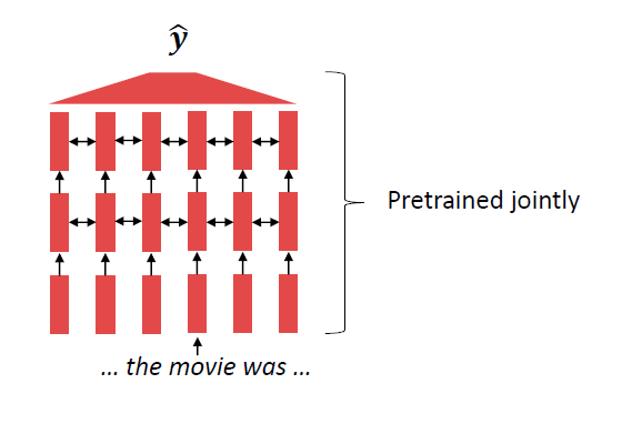
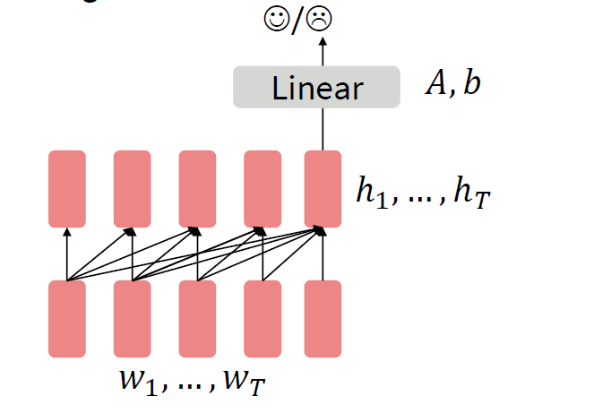
在读transformer论文的时候,有几个概念key,query,value三个概念一下子就抛出来了。在讲transformer的lecture video里,我看到有不少评论反应讲者没有将这三个概念讲清楚。我一开始在看cs231n的lecture ppt时也有点疑惑,老师刚说完general attention layer转到讲self-attention layer,就直接从h变成了q,确实有点云里雾里。
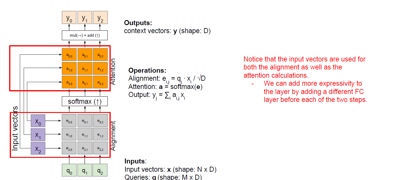
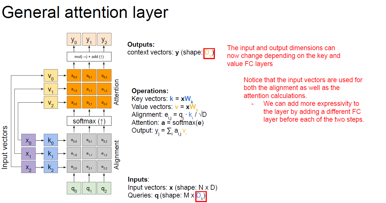
可以从上面的ppt中看出,原来是仅仅有q这个变量的,这是从一开始的h演变来的,而我们可以看到为了“add more expressivity to the layer”,所以我们在1.输入x输入到FC得到alignment score之前又加了一个不同的FC 2. 对输入x用attention weights进行weight sum的过程也加了一个完全不同的FC layer。而我们可以看到这里加的这两个FC layer是为了增加模型的表现力。这两个FC layer的输出也就是成了我们所说的key和value。后面的过程就清晰了,首先利用query和key计算attention weights,然后用attention weights和value进行计算得到context。
An attention layer does a fuzzy lookup like this, but it's not just looking for the best key. It combines the
valuesbased on how well thequerymatches eachkey.How does that work? In an attention layer the
query,key, andvalueare each vectors. Instead of doing a hash lookup the attention layer combines thequeryandkeyvectors to determine how well they match, the "attention score". The layer returns the average across all thevalues, weighted by the "attention scores