R-CNN vs SPP vs Fast R-CNN vs Faster R-CNN
最近在object detection任务上读这几篇文章,见识到神仙打架。一开始我只是关注image segmentation的任务,其中instance segmentation任务中Mask-RCNN是其中比较火的一个model,所以就把跟这个模型相关的几个模型都找出来看了看。这里想记录下这几天看这几篇论文的心得体会,如果有写的不正确的地方,欢迎批评指正。
其实去仔细看这几篇论文很有意思,梳理一下时间线就是:
2014年Girshick提出了RCNN,用于解决accurate object detection 和 semantic segmentation。该模型有一个drawbacks是每次一张图片输入进来,需要产生~2000个region proposals,这些region的大小都是不一致的,但我们对图片进行分类的下游网络都是需要fixed size的图片,那怎么办呢?作者提出使用wraped方法,具体可以参考作者的论文。总之最终我们输入到SVM也就是分类器的region图片大小都是一致的。
为了解决每次输入网络的图片大小怎么样才能变成fixed size的vector,2015年he kaiming提出了SPP(spatial pyramid pooling),跟前者RCNN不一样的地方在于:1) 将region proposal的方法用在了图片输入cnn网络得到的feature map上,2)从feature map选择出来的region proposal不还是不一样大小么?作者没有使用wrap的方法,而是提出了一个SPP layer,这个layer可以接受任何大小的图片,最终都会转化成一个fixed size的向量,这样就可以轻松输入进SVM或者Dense layer进行分类了。
收到SPP的启发,Girshick在2015年提出了Fast-RCNN,将SPP layer重新替换成ROI Pooling,经过ROI pooling,输出的并不是SPP layer输出的金字塔式的向量了,而是只有一个。 参考博客
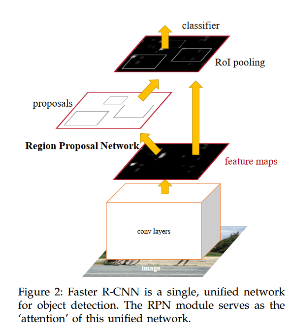
经过前一轮的battle,虽然各自的模型都提出了自己的独特方法,但是无论是SPP Net还是Fast-RCNN都没有提出在选择ROI(region of interest)的方法。2016年He Kaiming再次强势入场,提出了产生region proposal的方法,它使用了一个单独的CNN网络来获取region proposal.得到了这些proposal之后再将他们传递给Roi Pooling layer,后面的过程和fast RCNN一致。 这篇Faster-RCNN的方法作者中有he kaiming和Girshick,这里致敬下sun jian,感谢为computer vision领域贡献的灵感和创造。
Mask-RCNN
Mask-RCNN是Region-based CNN系列中的一个算法,用于解决instance segmentation的问题,instance segmentation的难点在于我们不仅要做object detection,而且需要将object的准确轮廓给识别出来,同时做出分类这是什么object。在Mask-RCNN
中,related work一章节对RCNN这一系列的模型做了准确概括,建议大家读原文:
The Region-based CNN (R-CNN) approach [13] to bounding-box object detection is to attend to a manageable number of candidate object regions [42, 20] and evaluate convolutional networks [25, 24] independently on each RoI. R-CNN was extended [18, 12] to allow attending to RoIs on feature maps using RoIPool, leading to fast speed and better accuracy. Faster R-CNN [36] advanced this stream by learning the attention mechanism with a Region Proposal Network (RPN). Faster R-CNN is flexible and robust to many follow-up improvements (e.g., [38, 27, 21]), and is the current leading framework in several benchmarks.
在Mask-RCNN的文章中提出了一种新的ROIAlign Layer,主要是为了解决Faster-Rcnn的网络中ROI pooling layer的问题。在此补充下ROI pooling是怎么将不同size的ROI(region of interest)都变成fixed-size的feature map的:
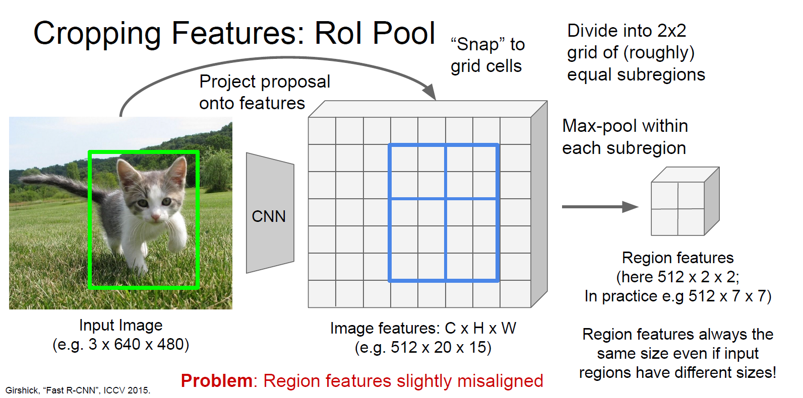
上图是将5*4大小的ROI变成了2✖2大小的feature map。这种方式带来的影响就是可能在提取的extracted features和ROI之间造成misalignments。但是这种misalignments并不会在faster-rcnn中对分类造成很大的影响,但如果要用这个ROI做segmentation的话就可能会造成巨大的影响,因此作者提出了一个ROIAlign Layer。
如果有小伙伴想对照code看这篇paper,可以参考tensorflow实现。如果你对pytorch更熟悉可以参考paper中给出的官方github地址的实现。有一篇博客详细介绍了tensorlfow的实现,参见blog
在MaskRCNN中使用了faster-rcnn中提出的RPN来产生ROI,然后才使用上面提到的ROI Algin。RPN的具体细节参见fatser-rcnn原文和本博客的第二章节
RPN(Region Proposal Network)
RPN 是在faster-rcnn中提出来的网络,主要是为了解决在rcnn和fast-rcnn两个前置模型中产生ROI的耗时问题,之前产生ROI主要是依靠Selected Search。在读mask-rcnn的paper时发现这个网络的细节不甚了解,这里补充记录一下。感兴趣的朋友可以阅读paper的第3.2节。
RPN在output长方体的ROI的同时,也会给每一个ROI产生一个Objectness score。看原文的时候作者是以sliding window的方式来讲解的,一开始看的有点懵。但其实就是卷积层的计算过程的拆解,我们先按照作者的思路来看RPN做了什么。
RPN的输入是经过一系列卷积层之后的feature map,在这个map上,我们在上面再做一些运算:
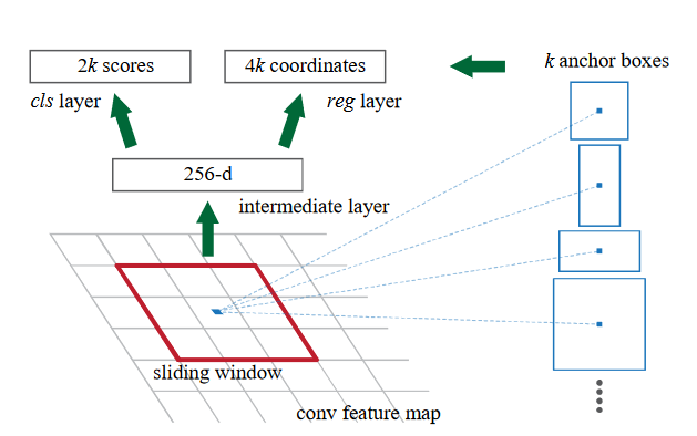
针对一个window(n✖n),RPN做的就是将这个window映射到一个低维度的feature上,图上是256维的向量,然后我们再接两个dense layer,一个用于预测box,一个用于做分类。k的意思是在每一个sliding window上我们都维护了k个anchor,这个概念和yolo里一致。所以在每一个sliding-window上我们都可以得出来4k个box和2k个分类结果(是否有object的概率),这个anchor box是和sliding-window的中心点绑定的,所以如果RPN的输入是一个W×H的feature map,那么我们就会有W×H×k个anchors。
那么我们知道RPN是怎么计算的了,然后在训练阶段还有一些tricks。作者对每一个anchor都赋予了一个class
label,赋予positive的anchor为 1) anchor和 groud truth的box有最高的IOU 2)
如果anchor与groud
truth的box的IOU大于0.7。这两种anchor都会被赋予positive的标签,也就是代表它里面有object。对于哪些和任何groud
truth
box的IOU都小于0.3的anchor,赋予negtive的标签。在为RPN产生训练数据时,对于所有的anchors都有一个class
label,也就是它里面是否包含object。对于box的训练数据的处理有一点不一样的地方。可以参考tensorflow实现,在mrcnn/model.py的build_rpn_target函数中:
1 | # RPN Match: 1 = positive anchor, -1 = negative anchor, 0 = neutral |
rpn_bbox的数量是提前设定好的,也就是不是对每一个anchor都会有一个box来对应,对于那些标记为positive的anchor box才会有bbox的target。
1 | # Generate RPN trainig targets |
输出为:
1 | target_rpn_match shape: (65472,) min: -1.00000 max: 1.00000 |
从上面可以看出,在全局变量设置中设置的是每一张图片最多有256个anchors,所以产生的rpn_bbox shape就是(256,4),而用于RPN训练的class label是全部的anchors的分类label。进一步的我们可以查看其中一张图片的anchors:
1 | positive_anchor_ix = np.where(target_rpn_match[:] == 1)[0] |
输出:
1 | positive_anchors shape: (14, 4) min: 5.49033 max: 973.25483 |
即便是有65472个anchors,但其实正负anchor所占比重很小,大多数是neutral的anchor。其中对于positive的anchor,我们拥有在他们的bbox上refine过的box。
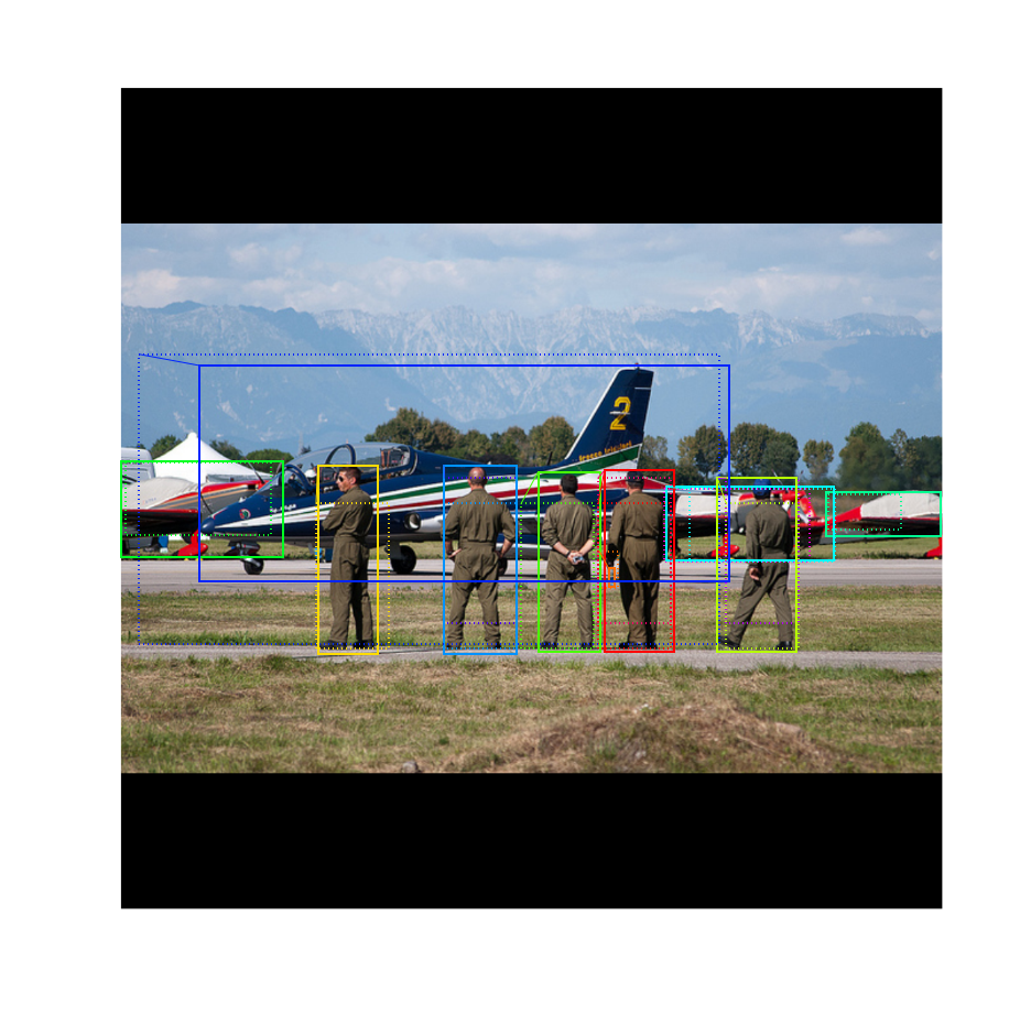
上图中虚线画出来的是positive anchor,实线框出来的是在这些anchor上refine过的box。
在训练阶段,计算loss时,对于regression loss,模型只会计算postive anchors的regression loss,也就是只计算那些被打上positive标签的anchor预测的box与groud-truth box的回归loss。如果一个anchor,它的class label在anatation阶段就是negtive的,模型并不会将它预测出来的box和ground-truth box进行比较,他们的loss不会被计算进总的Loss。
关于如何训练的问题,在Faster-Rcnn的文章中给出了三种训练的算法,第一种也是文中采用的方法就是:1. alternating training : 先把RPN单独训练,然后使用RPN产生的proposals去训练fast r-cnn. 然后将fine-tune过的RPN作为初始参数,然后再去产生proposal,再去训练fast rcnn. 具体来说就是4步:
- 单独train RPN : 用ImageNet pre-trained 参数做初始化,然后在region proposal这个task上fine tune
- 利用第一步产生的proposal训练Fast-Rcnn,也就是架构图中的最上面一部分,该网络也会使用ImageNet pre-trained 参数做初始化。注意一直到这一步,两个网络都没有share任何卷积layers
- 第三步我们使用detector的network去初始化RPN,同时fix住最下面的卷积层,也就是两个网络共享的那些卷积层。这一步骤单独fine-tune RPN的layers。
- 最后一步,fine-tune Fast-RCNN的unique的layers。