machine translation相关论文阅读
machine translation 这个任务一般是作为language modeling的紧接一个话题。它的前身(2010年之前)是statistical machine translation,但自从Neural machine translation出来之后,用statistical的方式来做translation就少了很多。有兴趣的可以了解下statistical machine translation的具体细节. 本博客主要记录NMT的主要论文和研究。NMT的架构主要是encoder-decoder架构,它其实是一个很典型的seq-to-seq的模型, 关于它的定义:
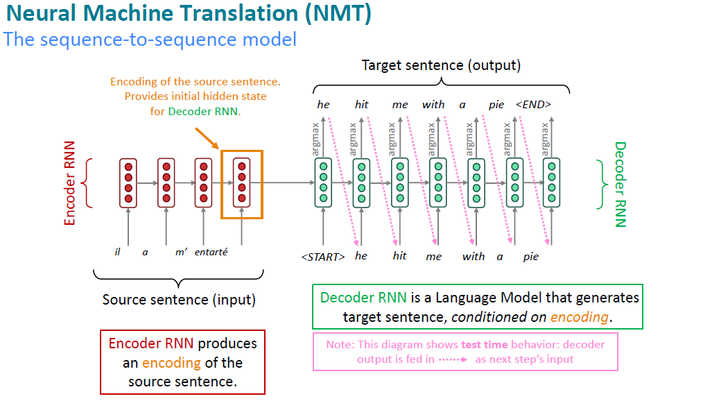
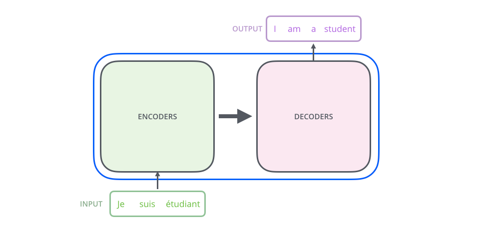
Neural Machine Translation (NMT) is a way to do Machine Translation with a single end-to-end neural network
它的一般架构是这样的:
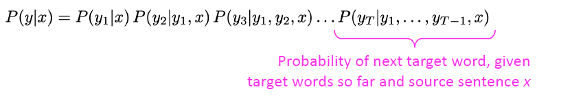
NMT所有的模型都基于一个统一的数学公式:
注意这里和statistical machine translation的公式是不一样的:
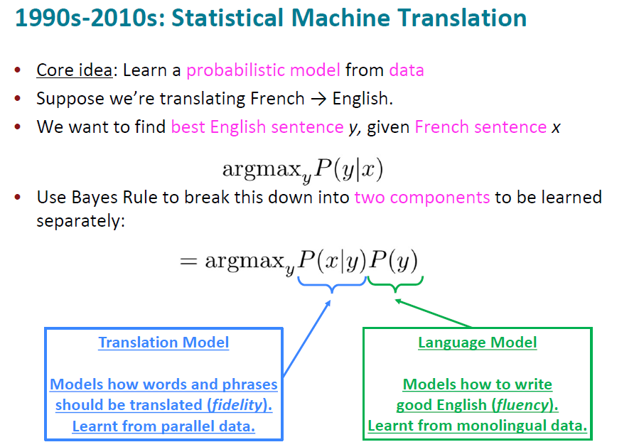
用统计翻译模型做的时候是分别解决translation model以及language model的问题,涉及很多特征工程的问题,很复杂。
在machine
translation领域,encoder-decoder架构的模型经历了好几次演变,最终才转化成加入了attention机制,模型架构的整理可以参考Neural Machine Translation: A
Review and
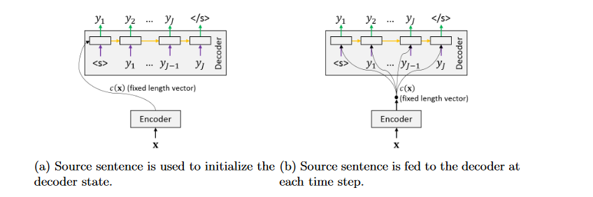
Survey。文章的第五章介绍了将encoder编码为固定长度的向量的用法。其中有两种使用这个C的用法,1.
作为decoder的初始化state 2.
作为decoder每一个时间步的固定输入和input一起去计算hidden state:
这些文章从Sequence to Sequence Learning with Neural Networks,再到Learning Phrase Representations using RNN Encoder-Decoder for Statistical Machine Translation. 然后就过度到attention时代了,所以作者在这篇review中只花了很少的第五章节就结束了。第六章就开始讲attentional encoder-decoder networks。
The concept of attention is no longer just a technique to improve sentence lengths in NMT. Since its introduction by Bahdanau et al. (2015) it has become a vital part of various NMT architectures, culminating in the Transformer architecture
这句话是6.1的精髓,attention的概念不再是我们上文所说的那些用于初始化呀,还是用作duplicate context。Bahdanau 2015年的这篇文章,也就是引入multi-head attention的这篇文章彻底打破了这个convention。因为我们可以看到transformer的架构中都没有RNN的身影,有的只是attention weights的计算。
Learning Phrase Representations using RNN Encoder-Decoder for Statistical Machine Translation 2014
这是在机器翻译领域encoder-decoder架构,在attention 机制提出之前表现最好的RNN模型。其实模型挺简单的,encoder负责将input sequence编码成了一个固定的向量Context,然后基于这个向量,decoder每一个时间步产生一个单词。在decoder的每一个时间步进行的运算是:
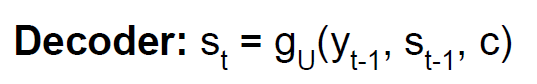
y_t是由s_t得到的。
同样的,这篇文章可以结合代码来看,轻易理解。该代码是用pytorch实现的。这个pytorch的实现是从Sequence to Sequence Learning with Neural Networks开始讲解的,Learning Phrase Representations using RNN Encoder-Decoder for Statistical Machine Translation这篇文章进步在

可以看到该篇文章介绍的模型优势在于预测y的时候加入了context以及\(y_{t-1}\),而不是仅仅依赖于\(s_t\)
以上的文章都是将input sentence编码成一个fixed-length的vector,从下面这篇2015年Bahdanau的文章开始,attention就开始用于NMT。为了解决fixed-length vector的问题,这样我们就不必要将input sentence的所有信息都编码到一个固定长度的向量里。
Neural Machine Translation by Jointly Learning to Align and Translate 2015
从这篇文章开始,attention的机制开始使用在翻译中。
在Introduction章节,最重要的一句话:
The most important distinguishing feature of this approach from the basic encoder–decoder is that it does not attempt to encode a whole input sentence into a single fixed-length vector. Instead, it encodes the input sentence into a sequence of vectors and chooses a subset of these vectors adaptively while decoding the translation
意即跟以往那种encoder-decoder的网络来做translation的model不同,虽然提出的模型也属于encoder-decoder架构,但不是将input sentence编码成一个固定长度的向量,而是将input sentence编码成一系列的向量并自适应的从中选择一个小子集的向量用来做decode。
截至文章发表,现有做机器翻译的模型中,表现最好的模型是RNN,内units用lstm。可以称之为RNN Encoder-Decoder。
还有一个发现是,这些encoder和decoder block,里面基本上是stacked rnns结构,也就是堆了好几层rnn。这个发现可以追溯到paper. 该作者发现在NMT任务上,high-performing rnns are usually multi-layer, 不仅如此,对于encoder rnn,2到4层是最好的,对于decoder rnn,4层是最好的。通常情况下,2层堆叠的RNN比一层RNN要lot better; 为了解决long dependency的问题,用lstm cell是必要的,但这也不够,需要使用一些其他的技术,比如skip-connection,dense-connections。
这里值得一提的是,虽然Bahdanau 2015年出的这篇文章很火。但是后来通过学习cs224n和观察tensorflow的文档:Neural machine translation with attention,发现luong 2015的这篇文章中的架构使用的更多,它的计算公式和Bahdanau介绍的有一点点不一样,再luong的文章中我们也可以看到它自己说的和Bahdanau不一样的地方:
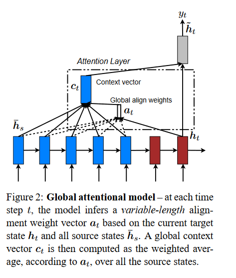
Comparison to (Bahdanau et al., 2015) – While our global attention approach is similar in spirit to the model proposed by Bahdanau et al. (2015), there are several key differences which reflect how we have both simplified and generalized from the original model. First, we simply use hidden states at the top LSTM layers in both the encoder and decoder as illustrated in Figure 2. Bahdanau et al. (2015), on the other hand, use the concatenation of the forward and backward source hidden states in the bi-directional encoder and target hidden states in their non-stacking unidirectional decoder. Second, our computation path is simpler; we go from ht → at → ct → ̃ ht then make a prediction as detailed in Eq. (5), Eq. (6), and Figure 2. On the other hand, at any time t, Bahdanau et al. (2015) build from the previous hidden state ht−1 → at → ct → ht, which, in turn, goes through a deep-output and a maxout layer before making predictions.7 Lastly, Bahdanau et al. (2015) only experimented with one alignment function, the concat product; whereas we show later that the other alternatives are better.
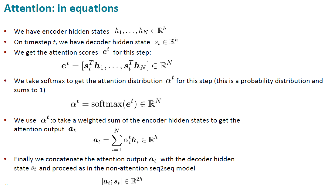
所以关于用attention来做machine translation的模型,我们只需要记住下面的计算过程就行,因为它也不是现在流行的machine translation的方法(毕竟2015年的时候transformer还没出来):
以上的模型给我们解决了标准的seq2seq的模型在做NMT任务时的一些问题:
- improves NMT performance
- provides more "human-like" model: replace the fixed length vector with dynamic vector according to the decoder hidden states
- solves the bottleneck problem: allows decoder to look directly at source
- helps with the vanishing gradient problem
- provides some interpretability
注意,虽然attention机制首先是在NMT任务中提出并得到了应用,但是它并不是seq2seq的专属,你也可以将attention用在很多architectures和不同的tasks中。有一个关于attention的更general的定义是:
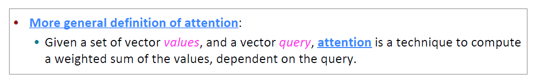
我们有时候会说: query attends to the values,例如在seq2seq2+attention的模型中,每一个decoder hidden state就是query,attends to 所有的encoder hidden states(values).
Attention is all you need 2017
在transformer的paper中,作者首先介绍本文:主流的sequence tranduction模型主要基于复杂的RNN或者CNN模型,它们包含encoder和decoder两部分,其中表现最好的模型在encoder和decoder之间增加了attention mechanism。本文提出了一个新的简单的网络结构名叫transformer,也是完全基于attention机制,"dispensing with recurrence and convolutions entirely"! 根本无需循环和卷积!了不起的Network~
在阅读这篇文章之前需要提前了解我在另外一篇博客 Attention and transformer model中的知识,在translation领域我们的科学家们是如何从RNN循环神经网络过渡到CNN,然后最终是transformer的天下的状态。技术经过了一轮轮的迭代,每一种基础模型架构提出后,会不断的有文章提出新的改进,文章千千万,不可能全部读完,就精读一些经典文章就好,Vaswani这篇文章是NMT领域必读paper,文章不长,加上参考文献才12页,介绍部分非常简单,导致这篇文章的入门门槛很高(个人感觉)。我一开始先读的这篇文章,发现啃不下去,又去找了很多资料来看,其中对我非常帮助的有很多:
- 非常通俗易懂的blog 有中文版本的翻译
- Neural Machine Translation: A Review and Survey 虽然这篇paper很长,90+页。前六章可以作为参照,不多25页左右,写的非常好
- stanford cs231n课程的ppt 斯坦福这个课程真的很棒,youtube上可以找到17年的视频,17年的课程中没有attention的内容,所以就姑且看看ppt吧,希望斯坦福有朝一日能将最新的课程分享出来,也算是做贡献了
- cs231n推荐的阅读博客 非常全面的整理,强烈建议食用. 这位作者也附上了自己的transformer实现,在它参考的那些github实现里,哈佛大学的pytorch实现也值得借鉴。
- The annotated Transformer 斯坦福出的关于Attention is All you need学术文章的解析以及代码实现,强烈建议食用。
Transformer这篇文章有几个主要的创新点:
- 使用self-attention机制,并首次提出使用multi-head attention
该机制作用是在编码当前word的时候,这个self-attention就会告诉我们编码这个词语我们应该放多少注意力在这个句子中其他的词语身上,说白了其实就是计算当前词语和其他词语的关系。这也是CNN用于解决NMT问题时用不同width的kernel来扫input metric的原因。
multi-head的意思是我使用多个不同的self-attention layer来处理我们的输入,直观感觉是训练的参数更多了,模型的表现力自然要好一点。
- Positional embeddings
前一个创新点解决了dependence的问题,那如何解决位置的问题呢?也就是我这个词在编码的时候或者解码的时候应该放置在句子的哪个位置上。文章就用pisitional embedding来解决这个问题。这个positional embedding和input embedding拥有相同的shape,所以两者可以直接相加。transformer这篇文章提供了两种encoding方式:
1) sunusoidal positional encoding
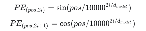
其中,pos=1,...,L(L是input句子的长度),i是某一个PE中的一个维度,取值范围是1到dmodel。python实现为:
1 | def positional_encoding(length, depth): |
2) learned positional encoding
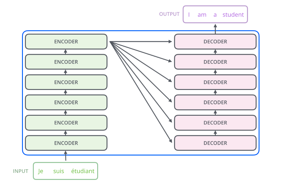
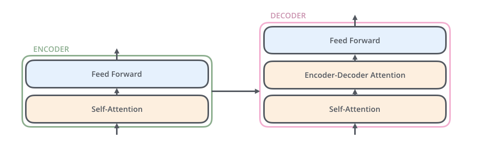
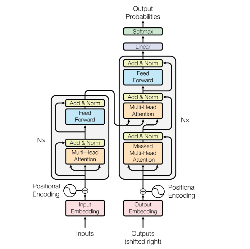
整体上看,这篇文章提出的transformer模型在做translation的任务时,架构是这样的:
其中encoders部分包含了6个encoders的block,decoders部分也包含了6个decoders的block,将encoders的每一个block拆开来看,有两个sub layer:
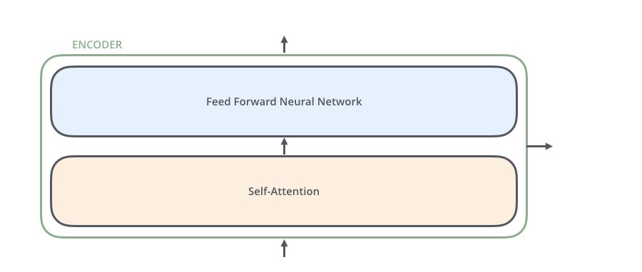
其中decoder部分的block比encoder部分的block多了一个sub layer,其中self-attention和encoder-decoder attention都是multi-head attention layer,只不过decoder部分的第一个multi-head attention layer是一个masked multi-head attention,为了防止未来的信息泄露给当下(prevent positions from attending to the future).
在transformer模型中,作者还使用了residual connection,所以在encoder的每一个block中,数据的flow是:
其中self-attention中涉及的运算details是:
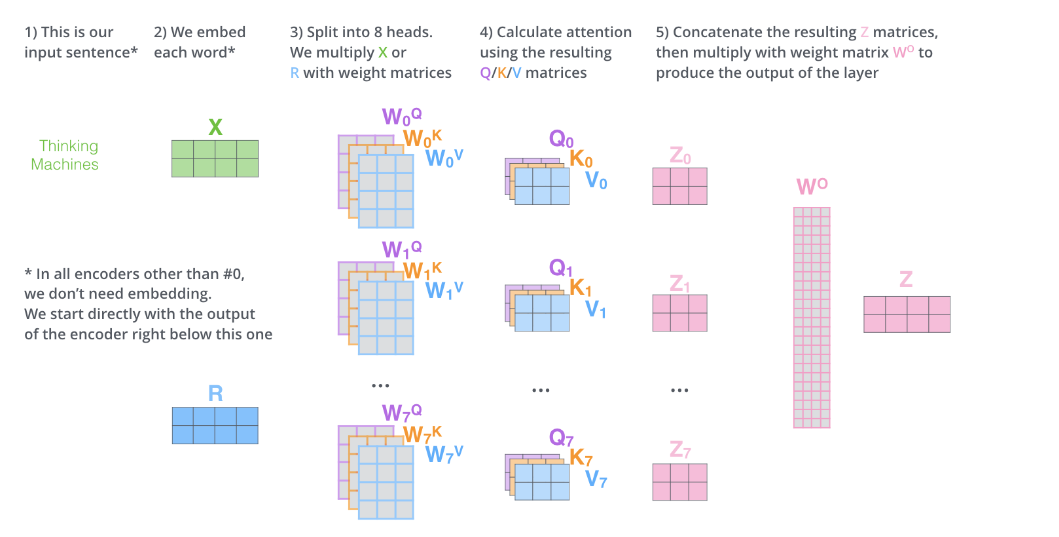
可以发现其中涉及的运算都是矩阵的点乘,并没有RNN中那种时间步的概念,所以所有运算都是可以parallelizable,这就能使得模型的推理和训练更加的efficient。并且!Transformers也可以抓住distant的依赖,而不是像rnn那样对于长依赖并不是很擅长,因为它前面的信息如果像传递到很后面的单词推理上,需要经历很多时间步的计算,而transformer在推理每一个单词的时候都可以access到input句子中的每一个单词(毕竟我们的Z中包含了每一个单词跟其他单词的关系)。
其中positional encoding现在可以简单的理解成在我们编码的word embedding上我们又加了一个positional encoding,维度和我们的embedding一模一样。
在tensorflow中有一个layer是
MultiHeadAttention,如果我们想实现transformer里的这个self-attention,那就是query,key,value其实都是由input vector计算来的。
以上的理论计算看起来可能会有点模糊,可以同步参照博客 参考 illustrated transformer介绍的详细细节,基于tensorflow框架实现的transformer来帮助自己理解transformer模型。
encoder部分
encoder的每一个block由两个sub-layer组成,中间穿插resnet connection。
![]()
1 | def multihead_attention(self, query, memory=None, mask=None, scope='attn'): |
decoder部分
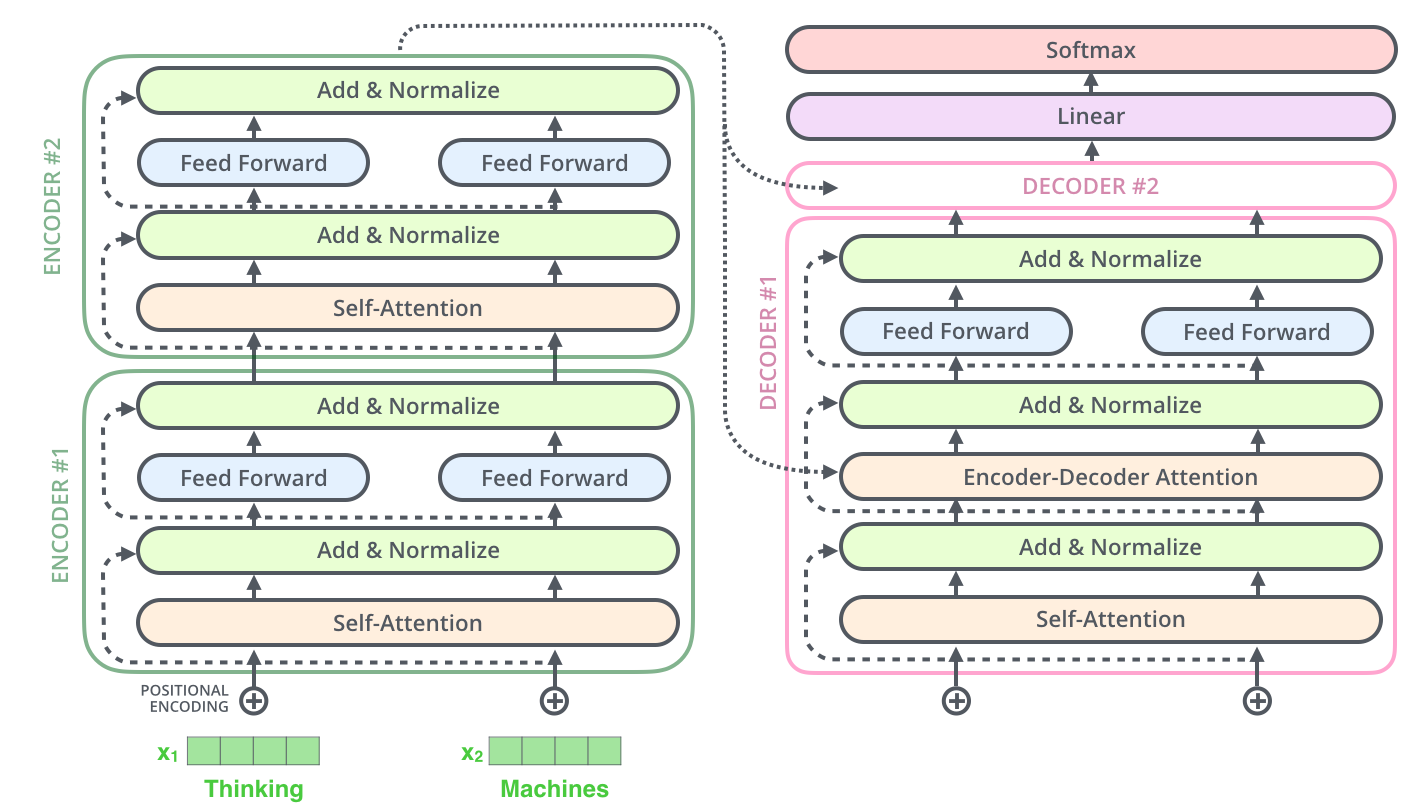
在decoder部分,我们可以看到每一个decoder block的输入有两个:整个encoder部分的输出以及上一个decoder block的输出(第一个decoder block是词向量的输入),而encoder部分的输出是接到每一个decoder block的第二个sublayer的。正如刚刚提到了,decoder部分的每一个block跟encoder部分的block有一个不一样的地方,那就是多了一个sublayer: encoder-decoder attention。至于encoder部分和decoder部分是如何connect的,
The encoder start by processing the input sequence. The output of the top encoder is then transformed into a set of attention vectors K and V. These are to be used by each decoder in its “encoder-decoder attention” layer which helps the decoder focus on appropriate places in the input sequence
也就是我们得到了encoder部分top layer(最后一个encoder
layer)的输出之后,我们将输出转化成K和V.
我们可以看到在multihead_attention里,memory是enc_out
1 | def decoder_layer(self, target, enc_out, input_mask, target_mask, scope): |
以上实现的transformer其实我觉得还是有一点点复杂,毕竟在tensorflow2.0+版本中已经有了官方实现好的layers.MultiHeadAttention可以使用,应该可以大大简化我们实现步骤,特别是上面的def multihead_attention(self, query, memory=None, mask=None, scope='attn'):。从刚刚的实现里我们可以发现,除了decoder部分每一个block的第二个sublayer的attention计算有一点不一样之外,其他的attention计算都是一模一样的。我在github上找了不少用TF2.0实现的transformer(最标准的也是Attention
is all you
need的模型),发现很多都都写得一般般,最终发现还是tensorflow官方文档写的tutotial写的最好.
现在对照tensorflow的tutorial以及上面transformer的计算过程,拆解一下官方给的代码。
首先定义一个baseAttention类,然后在此基础上我们再定义encoder和decoder中的attention:
1 | class BaseAttention(tf.keras.layers.Layer): |
那么针对encoder结果输入到decoder的cross attention layer怎么处理呢?这时候我们使用MultiHeadAttention时就需要将target sequence x当作是query,将encoder输出当作是context sequence也就是key/value。
1 | class CrossAttention(BaseAttention): # encoder结果输入到decoder的层 |
然后我们再定义global attention,global attention就是没有任何特殊操作的(比如上面的attention计算它有特别的context),而在transformor中更多的是self-attention,也就是我们传递给MultiHeadAttention的query,key,value都是同一个值。
1 | class GlobalSelfAttention(BaseAttention): |
最后我们定义causal self attention layer,这个是在decoder的每一个block的第一个sublayer:self-attention layer.其实这个layer是和global attention layer差不多的,但还是有一点微小的差别。为什么呢?因为我们在decoder阶段,我们是一个词语一个词语的预测的,这其实包含了一层因果关系,我们在预测一个词语的时候,我们应该已知它前面一个词语是什么,RNN中的hidden state传递到下一个时间步就是这个因果关系的传递。那么如果我们使用刚刚我们实现的global attention layer来实现这个self attention,并没有包含这个因果关系,不仅如此,如果我们使用常规的self attention的计算,将target sequence全部当作输入输入到decoder中的第一个block中,会有未来的数据提前被当前时刻看到的风险,所以在Transformer这篇文章中,作者提出使用mask的技术来避免这个问题。
在tensorflow中实现很简单,就只需要给MultiHeadAttention传递一个use_causal_mask = True的参数即可:
1 | class CausalSelfAttention(BaseAttention): |
这样就可以保证先前的sequence并不依赖于之后的elements。这里我本来有一个疑问是,这样一来这个causal layer并不能实现bi-rnn的能力?但后来一想并不是,因为双向的RNN的后向是指后面的词语先输入,其实就是从后往前输入,这样就可以知道一个sequence当前词语依赖于后面的词语的权重。
补充介绍
tf.keras.layers.MultiHeadAttention
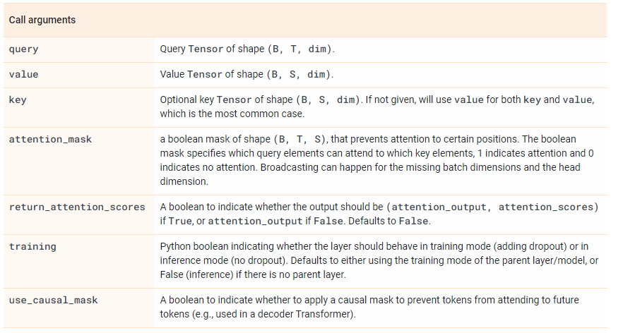
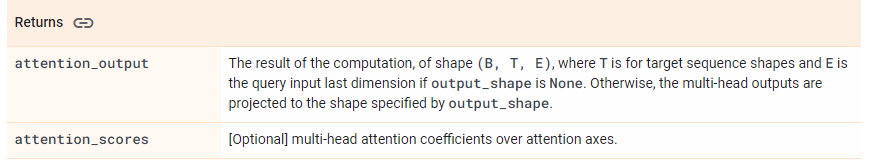
注意,return的结果包含两个,其中attention_output的shape的第二维是和target sequence的长度是一致的,并且E是和query的最后一维是一致的。
Attention Family
这个章节整理于blog,这个作者之前写了一篇介绍attention的文章,后面在2023年一月的时候又更新了两篇博客,详细介绍了从2020年以来出现的新的Transformer models。权当自己学习记录一些我还需要补充的知识。
The Transformer (which will be referred to as “vanilla Transformer” to distinguish it from other enhanced versions; Vaswani, et al., 2017) model has an encoder-decoder architecture, as commonly used in many NMT models. Later simplified Transformer was shown to achieve great performance in language modeling tasks, like in encoder-only BERT or decoder-only GPT.