Novel view synthesis(NVS)
New Topic For Me to explore! 对我来说正式开启3D Image~
首先我是看了两篇review了解了这个topic的主要任务:
- advancements in radiance field techniques for volumetric video generation: a technical overview
- From Capture to Display: A Survey on Volumetric Video
另外同步阅读了huggingface的tutorial:https://huggingface.co/learn/computer-vision-course/unit8/3d-vision/nvs 。这篇博客将NVS描述为这样一个任务:
generate views from new camera angles that are plausibly consistent with a set of images.
我们在对一个场景进行3D还原时,首先的输入是一系列相机在不同的视角拍摄的静态图片,通过这些图片我们对该场景下的人物以及物体进行3D建模,但相机个数是有限的,如何推算出某个没有相机的角度上的view,这就是NVS这个任务要做的事情。
很多方法在这个topic上提出来,大致可以分成两类:1)generate an intermediate three-dimensional representation, which is rendered from a new viewing direction. 比如PixelNeFRF 2)direclty generated new views without an intermediate 3D representaion, 比如Zero123
2025.6.24 补充
对于该领域的scene的生成,24年google的4D Gaussian Splatting提出后,把NVS分为两部分,一部分是以Nerf和3DGS为代表的基于静态图片生成3D场景,另外一部分是dynamic scenes,这里的dynamic指的是与3DGS处理的某一时刻的scene不同,这里要处理的数据加入了时序特征,场景中有动态的物体或者人,比如行人或者行驶的车辆。4DGS在一定程度上解决了真正的real-time的问题。
NeRF
NeRF: Representing Scenes as Neural Radiance Fields for View Synthesis
2020年出的一篇文章,下面这句话就是它这个算法的精华:
Our algorithm represents a scene using a fully-connected (nonconvolutional) deep network, whose input is a single continuous 5D coordinate (spatial location (x, y, z) and viewing direction (θ, φ)) and whose output is the volume density and view-dependent emitted radiance at that spatial location
LLFF 数据集
在查看NeRF的github code(Pytorch)时,也有tensorflow版本,移步官方repo。发现作者使用了两个数据集,其中一个就是LLFF,本着学习的原则,先把LLFF数据集搞清楚。
LLFF全称为Local light Field Fusion,也是提出了一个NVS的算法。LLFF的主旨思想是:
present a simple and reliable method for view synthesis from a set of input images captured by a handheld camera in an irregular grid pattern.
简单说就是:该方法可以从一系列手持拍摄的静态图片生成一个scene,这个scene可以理解为一个3D的场景,可以用VR眼镜看的那种。
该LLFF repo提供了非常详细的安装教程,令我比较感兴趣的是,它可以基于自己拍摄的一些静态图片生成一个scene。先来看看它的这份代码。
我们的输入是从一系列的images开始的,首先第一步
- recover cammera poses
这一步采用COLMAP 实现了一个 struture from emotion的pipeline。这一步的输入是一系列的静态图像,输出的是这个场景下的 6-DoF camera poses和 near/far depth bounds。
Structure-from-Motion (SfM) is the process of reconstructing 3D structure from its projections into a series of images. The input is a set of overlapping images of the same object, taken from different viewpoints. The output is a 3-D reconstruction of the object, and the reconstructed intrinsic and extrinsic camera parameters of all images.
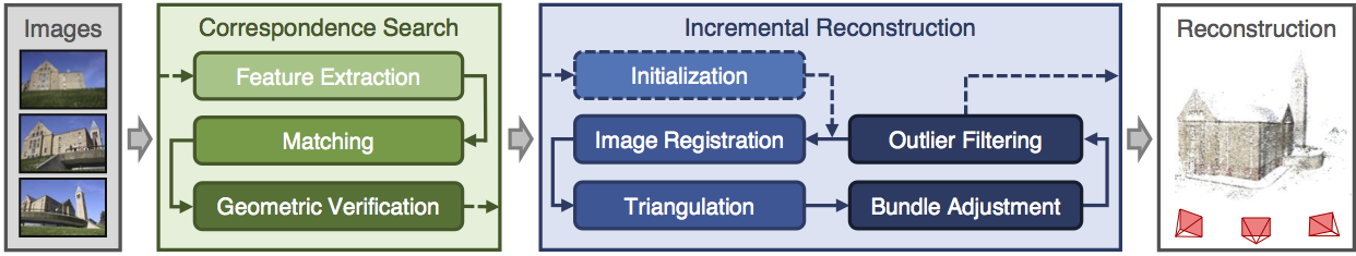
COLMAP使用的方法依赖于Structure-from-Motion Revisited这篇文章,它将SfM分成三个步骤:
- feature detection and extraction
这一步好理解,特征抽取,利用一个apprearance descriptor f
- feature matching and geometric verification
feature matching利用前一步的features找出这一系列图片中的same scene part。原文是这样写的:
The na ̈ıve approach tests every image pair for scene overlap; it searches for feature correspondences by finding the most similar feature in image I(a) for every feature in image I(b), using a similarity metric comparing the appearance fj of the features
简单理解就是根据上一步抽取的features去一一比对每一对image pair,寻找出每一对image pair中的相似feature,从而找出same scene part。
geometric verification 我觉得有点稍微难理解。上一步只是确认了每一张图片中在apperance上相似的scene part,但有可能不是指代的这个场景下的同一个object(Point), 所以就需要去verify上一步的match是否准确,怎么verify呢?通过projective geometry去预估transformation
Since matching is based solely on appearance, it is not guaranteed that corresponding features actually map to the same scene point
- structure and motion reconstruction
LLFF中实现上述第一步骤的脚本为imgs2poses.py,
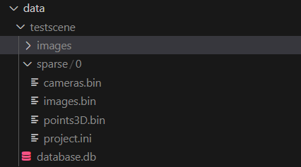
看该源代码就是基于COLMAP来做的。试着运行该脚本,测试数据用repo内的download_data.sh下载的数据。运行完后可以看到如下输出:
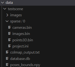
其中images是source images,testscene下除了images这个文件夹,其他都是COLMAP生成的。具体含义参考COLMAP的document
logs文件内容:
1 | Need to run COLMAP |
仔细分析一下imgs2poses.py,一共用COLMAP执行了三条terminal命令:
1 | # extract features |
对照colmap cli的guidebook,
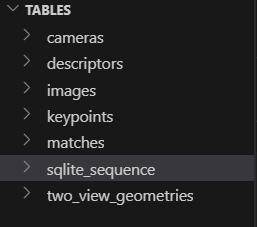
作者使用了前三个命令,dense部分没有继续生成。想要知道它output出来的这些.bin文件含义,需要搞明白database.db内有什么东西,它是feature
extraction的产物。db文件可以用vscode的插件打开,它包含7个table:
keypoints表格中,我下图截图的data部分里才是所有feature的信息,内有每一个feature所在的X,Y坐标。
COLMAP uses the convention that the upper left image corner has coordinate (0, 0) and the center of the upper left most pixel has coordinate (0.5, 0.5)
COLMAP在表示图像坐标时,采用了一种特定的坐标系统,其中图像的左上角被定义为坐标原点 (0, 0)。而“the center of the upper left most pixel has coordinate (0.5, 0.5)” 指的是图像中最左上角的像素的中心位置被赋予了坐标 (0.5, 0.5)。
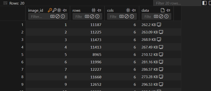
在这两张表格中,rows表示的数值是number of detected features per image, 如果rows=0, 那么这个image没有feature
在运行命令colmap exhaustive_matcher --database_path ./data/testscene/database.db后,db文件内的matchs这张表会出现值(之前没有),每一行会表示一张图片和另外一张图片的匹配结果,rows的值表示match上特征点的个数。
第三个命令colmap mapper...实现了sparse
3D的重建,在前面两个命令产生的结果上(feature
extraction&match)。运行完第三条命令后,文件夹内的内容是这样的:
第三条命令产生的结果放在sparse文件夹内。
如果用LLFF
repo内的imgs2poses.py,脚本运行后会发现在testscene文件夹下还会出现一个poses_bounds.npy的文件,查看imgs2poses.py中的gen_poses方法,会发现在执行完colmap的上面三条命令后又再次运行了load_colmap_data()和save_poses()。其中的load_colmap_data()对colmap三条命令的结果,也就是三个bin文件做了读取和处理:
1 | def load_colmap_data(realdir): |
这里readme中也对pose_bounds.npy的内容进行了解释。这个文件很重要,可以看到nerf中导入LLFF数据集也是从该文件中导入的数据,导入方式只有三行代码:
1 | poses_arr = np.load(os.path.join(basedir, 'poses_bounds.npy')) |
我本来也是先看的nerf的代码,看到这里导入LLFF数据集的方式没看懂,主要是不知道pose_bounds.npy内存储的内容的具体含义,所以才补充了LLFF的上面的诸多知识空白。LLFF的作者在readme中对这个文件的含义进行了解释:
This file stores a numpy array of size Nx17 (where N is the number of input images).Each row of length 17 gets reshaped into a 3x5 pose matrix and 2 depth values that bound the closest and farthest scene content from that point of view.
这里有一个比较重要的概念”相机的姿态“(cammera poses),可以参考阅读:
其中
T_{cw}为该点从世界坐标系变换到相机坐标系的变换矩阵,T_{wc}为该点从相机坐标系变换到世界坐标系的变换矩阵。它们二者都可以用来表示相机的位姿,前者称为相机的外参。实践当中使用
T_{cw}来表示相机位姿更加常见。然而在可视化程序中使用T_{wc}来表示相机位姿更为直观,因为此时它的平移向量即为相机原点在世界坐标系中的坐标。视觉 Slam 十四讲中的第五讲的 joinMap 使用的就是T_{wc}来表示相机位姿进行点云拼接。
poses = poses_arr[:, :-2].reshape([-1, 3, 5]).transpose([1,2,0])
取前15个数,去掉最后2个near和far,并reshape成(N,3,5)的矩阵:
┌ ┐ │ R11 R12 R13 t1 hwf1 │ │ R21 R22 R23 t2 hwf2 │ │ R31 R32 R33 t3 hwf3 │ └ ┘
其中R部分是旋转矩阵,t是平移向量。
最终
poses.shape = (3, 5, N),其中:
poses[:, :4, :]→3x4的 相机外参 (R|t)poses[:, 4:5, :]→3x1的 相机内参[h, w, f]
bds = poses_arr[:, -2:].transpose([1,0]):取出
最后两列,即 near 和 far
深度边界,形状是 (N, 2)。
.transpose([1,0]):交换轴顺序,使
bds.shape = (2, N):
- 第一维 (2):表示 最近 (
near) 和 最远 (far) 深度 - 第二维 (N):对应 N 张图像
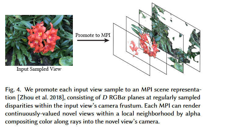
- Generate MPIs
脚本为imgs2mpi2.py。这一步是采用训练好的tensorflow模型对第一步骤的结果进行MPI的生成。这一步实现的结果如下:
Nerf Code 解析
回到Nerf的pytorch代码。train()中args可以指定输入哪一种数据集,我们这里就只看llff,
首先是load_llff_data:
1 | images, poses, bds, render_poses, i_test = load_llff_data(args.datadir, args.factor, |
images: 图像数据
poses: 相机姿态矩阵
bds: 每个图像的深度范围
render_poses: 渲染路径相机姿态(用于可视化)
i_test: 被选为 holdout 的视角索引(用于验证)
poses的shape为 [N_images, 3, 4],每一个poses[i] 是一张图像的相机外参矩阵(camera-to-world)。 \[ pose=[R t] \]
- R:旋转矩阵(表示相机朝向)
- t:平移向量(相机在世界坐标中的位置)
📌 它告诉你:这张图像的每一条光线从哪里发出,朝哪个方向发射。
我们知道nerf的输入是一个5D的输入
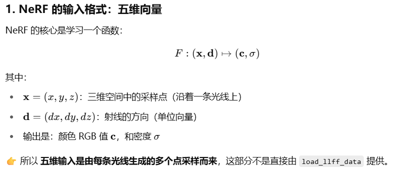
有了poses之后,下面的步骤就是: 像素 → get_rays → rays_o, rays_d ↓ 在光线上采样 t 值 (near → far) ↓ points = rays_o + t * rays_d ↓ 每个点输入 MLP → 得到 (σ, RGB) ↓ 体渲染(volume rendering) → 聚合颜色 → 图像像素
其中get_rays()就是对该图片上每一个像素点形成的时候的光线,该函数会返回每一条光线的起点和防线:
1 | rays_o, rays_d = get_rays(H, W, K, torch.Tensor(pose)) # (H, W, 3), (H, W, 3) |
注意这里的shape是(H,W,3),H是该image的高度,W是该image的宽度。3是表示三维里的坐标,rays_o基本一致,都表示相机位置。
既然对每一个像素有了一条射线,下面要做的就是在每一个射线上sample好多个点,如paper中图画的:
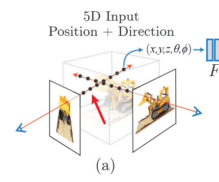
这一步在代码中是render()做的,render接受的一个输入参数是rays,rays中包含了选取的的射线的起点以及方向。函数内具体操作的这一部分在render_rays()内。
射线上采样:
1 | python复制编辑z_vals = torch.linspace(near, far, N_samples) # (N_samples,) |
将采样的点输入网络
1 | raw = network_fn(pts_flat) # MLP 输出密度 σ 和颜色 RGB |
这里的 pts_flat 是把 pts
拉成二维形状:(N_rays * N_samples, 3)
如果有 viewing direction,还会加到 MLP 输入中。
volume rendering
根据每个点的预测密度σ 和颜色 c,使用体渲染公式:
1 | T_i = exp(-∑_{j=1}^{i-1} σ_j * Δ_j) # 累积透射率 |
3DGS
自从3DGS出来之后,nerf上的更新就变少了,基本上是3DGS的天下了,3DGS的原文很难读懂,code也是比较难的,我找了很多其他的博客来理解它和nerf的区别,这里推荐几个。
- Talk | 加州大学洛杉矶分校周诗杰:3DGS时代的三维场景表示与生成 中文,视频前20分钟解释了3DGS的一些原理,它的泼墨比喻还挺形象的,虽然我还是没怎么明白其中细节,这位presenter主要是为了讲自己的工作,当作3DGS的引言好了。其中这位博主解释了为什么叫novel view (新颖视角).
- Three Level Summary: Neural Radiance Fields vs. 3D Gaussian Splatting 解释3DGS和nerf区别的,通俗易懂,建议阅读。一些重点地方我也贴上了,这些话很好的帮助我理解了3DGS。
The goal of both NeRFs and 3DGS is to solve the following problem: given a few images of some 3D scene taken from different camera viewpoints, can we generate an image of this scene from any new camera viewpoint? This problem is formally called novel view synthesis, since we’re attempting to synthesize (generate) novel (new) views of some particular scene.
3DGS builds on rasterization. The 3DGS algorithm essentially learns a point cloud of splats3 (ie. ellipsoids, or mathematically, 3D Gaussians) from input images, and once the point cloud is learned, you can place your camera wherever you want to view the point cloud from a novel view. Here’s some very high-level pseudocode to train 3DGS:
2
3
4
5
6
7
8
9
10
11
While average loss > threshold:
For each input image:
Generated image = Rasterize(splats)
Loss = Generated image - input image
If a splat doesn't cover enough space in an area:
Clone a new splat in the area
If a splat covers too much area:
Split that splat into two
For each splat:
Modify splat parameters to reduce loss
No neural networks are used for 3DGS; instead, the algorithm iteratively learns to clone, split, or modify (ex. change the size or color of) splats based on the loss4, until the generated images look similar to the input images.
大抵上,3DGS包含四个步骤:
- Struture from motion
该步骤用colmap处理一系列多视角的静态图片,colmap最终会输出一个简易point cloud作为3DGS的初始输入,nerf的初始化也是colmap生成的这个点云
- Convert to gaussian splats
这一步会将第一步生成的点云转化为高斯splats, 以供后续的rasterization。这些splats是一系列参数,这些参数存储着: 位置信息, splat的大小,透明度,颜色, 材质(material properties)。
- Training
3DGS的训练方式其实和nerf差不多,包含一个前向传播以及backwords loss。
前向传播就是将一个3D Gaussian映射到一个2D平面上(camera plane),这个过程是3D gaussian转化为2D Gaussian的过程,最终的image是由2D gaussians计算而来(Depth compositing of gaussians)。
Loss: 既然我们有了前述前向传播得出来的某个视角下的image,我们将该image和GT Image进行pixel的比对,就得到每一个loss对于每个pixel的gradient, 接下来的过程就比较熟悉了,就利用chain rule求对于输入参数,也就是3D gaussians的参数的导数就行。具体的数学推导可以参考 Mathematical Supplement for the gsplat Library。
- Differentiable gaussian rasterization
rasterization 表示的是forward pass这个过程。
3DGS Code 解析
这里我看的是3DGS的官方repo
首先先对该场景初始化一堆的gaussian, 初始化完成后就可以得到该场景了:
1 | gaussians = GaussianModel(dataset.sh_degree) |
然后是随机选取训练集中的某个视角,对该视角下的2D图片进行“推理”,也就是render:
1 | for iteration in range(first_iter, opt.iterations + 1): |