Prompt Engineering, also known as In-Context
Prompting, refers to methods for how to communicate with LLM to
steer its behavior for desired outcomes without updating the
model weights. It is an empirical science and the effect of prompt
engineering methods can vary a lot among models, thus requiring heavy
experimentation and heuristics
2013年的综述文章A Survey of
Large Language Models 在第五章介绍了详细的adaptation tuning of
LLMs的方法,也就是我一个pretrain好的LLM,如何让它在不同的任务上得到更好的泛化能力,这时候就要tuning
LLM。作者介绍其中有两种方法,一个是instruction Tuning,第二个是alignment
tuning。后者就是利用增强学习让模型从人类的反馈中去改进自己生成的文本,InstructGPT采用了这种方法。第一种会稍微复杂一点,但原理很简单,就是创造一系列的instruction和问答对,让LLM在这些新instruction上重新finetune,loss为sequence-to-sequence的loss。
[My personal spicy take]
这里这篇综述我觉得写的不完整,有点误导读者。这篇综述第五章只介绍了adaptation
tuning模型中的两种,但在instruction
tuning出现之前,还有不少技术能够帮助我们“further adapt LLM according to
specific goals”. 不仅如此,这篇综述也没有很好的解释instruction
tuning为什么就能帮助我们在不同任务上有了performance的提高。所以我就想写一篇博客来记录如果我们拥有了一个pretrained的大模型,我们可以有什么样的做法来使得大模型在特定的任务上为我们所用。详见另一篇博客“Adaptation
Tuning of LLMs”
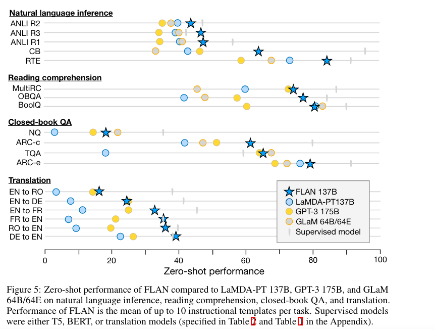
在接触羊驼模型后,我一直有一个疑问,为什么instruction
finetuned模型performance有了提高,或者说它在什么样的任务上有了提高?这个问题一直困扰我,直到我看到了google家的Finetuned Language Models Are
Zero-Shot Learners.instruction
tuning这种finetune方式的提出是为了improve zero-shot performance
on unseen tasks,具体一点就是在一些任务上比如阅读归纳,question
answering和语言推理上,研究者发现GPT3的zero-shot learning比few-shot
能力差很多,作者说一个潜在的原因是因为如果没有一些context给到模型的话,模型在面对跟pretrain时候数据相差很大的prompt时候会很困难,说直白点,就是没有例子给它参考了,就不会做题了。instruction
tuning这种方式就提供了一种非常简单的方式,它在好多个task上finetune这个模型,这里每一个task的数据组织形式跟原来不一样了,现在被组织成了(instruction,[input],output)的形式。finetune完之后的模型在unseen
task上做evaluation,研究者发现被instruction
finetune之后的模型比原来的模型在同一任务上的zero-shot能力大大提升:
performance
instruction tuning
想要做到instruction tuning有两个前提条件:1. 你有一个pretrained的模型
2.
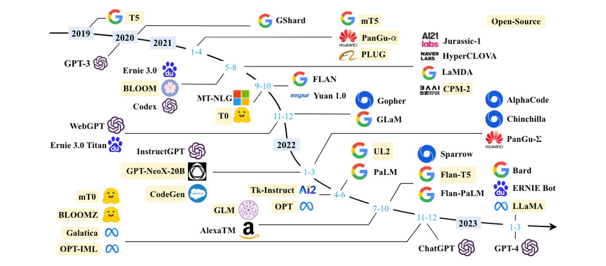
有很多instructions。首先第一个条件可以看看市面上有哪些模型是已经开源了,参考A Survey of Large Language
Models3.1的整理,2023年斯坦福的羊驼模型是基于meta的LLaMA,所以目前github上出现了很多用LLaMA为LLM,在上面做instruction
tuning工作的。
LLMs
那第一个问题解决了,起码我们有开源的LLM可以load到本地来使用,感谢facebook的开源。第二个问题如何产生很多的instructions,斯坦福的羊驼模型Alpaca采用的是下面文章介绍的方法,省时省力,花费上不超过600美金。当然也有其他的一些产生instruction的方法,详细可以参考A Survey of Large Language
Models
,其中作者介绍了一系列可以从现有数据集生成instruction的方法,这些方法应该也是低成本快速产生instruction的方法。
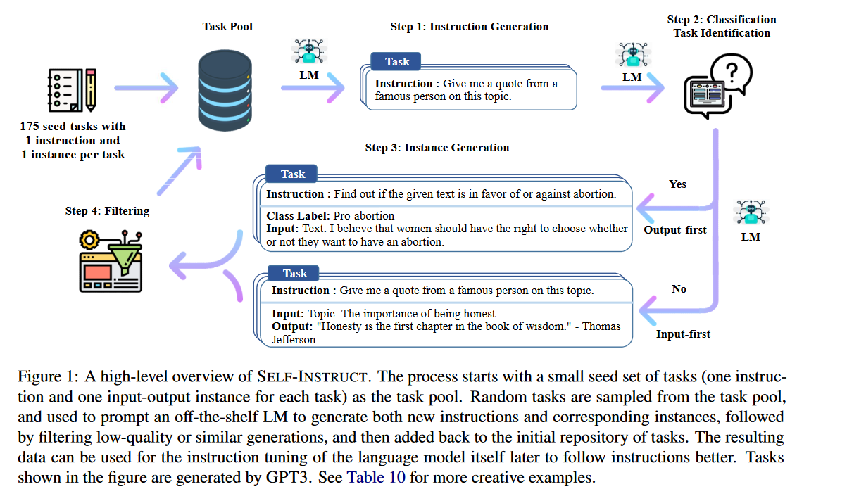
Self-instruct: Aligning
Language Model with Self Generated Instructions
这篇文章介绍了一种self generated
instructions的方法,简单说就是让LLM自己生成人类的问题的答案,然后将这些instructions
重新来fine-tune我们的LLM。这样做的一个前提条件是:1. Large
“instruction-tuned” language models (finetuned to respond to
instructions) have demonstrated a remarkable ability to generalize
zero-shot to new tasks. 2. 产生instruction
data非常的耗时,原来都是采用Human written的方式。具体步骤是:
The concept of attention is no longer just a technique to improve
sentence lengths in NMT. Since its introduction by Bahdanau et al.
(2015) it has become a vital part of various NMT architectures,
culminating in the Transformer architecture
同样的,这篇文章可以结合代码来看,轻易理解。该代码是用pytorch实现的。这个pytorch的实现是从Sequence to Sequence Learning
with Neural Networks开始讲解的,Learning Phrase Representations
using RNN Encoder-Decoder for Statistical Machine
Translation这篇文章进步在
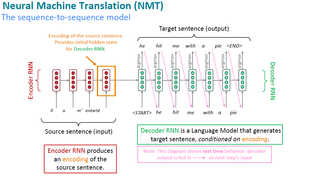
Neural
Machine Translation by Jointly Learning to Align and Translate 2015
从这篇文章开始,attention的机制开始使用在翻译中。
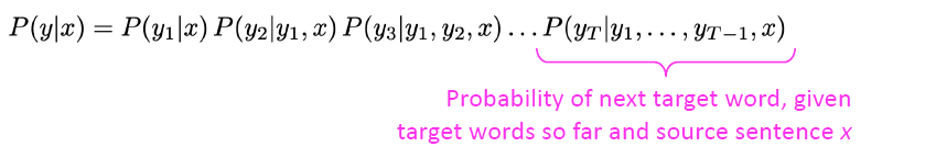
在Introduction章节,最重要的一句话:
The most important distinguishing feature of this approach from the
basic encoder–decoder is that it does not attempt to encode a whole
input sentence into a single fixed-length vector. Instead, it encodes
the input sentence into a sequence of vectors and chooses a subset of
these vectors adaptively while decoding the translation
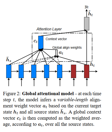
Comparison to (Bahdanau et al., 2015) – While our global attention
approach is similar in spirit to the model proposed by Bahdanau et al.
(2015), there are several key differences which reflect how we have both
simplified and generalized from the original model. First, we simply use
hidden states at the top LSTM layers in both the encoder and decoder as
illustrated in Figure 2. Bahdanau et al. (2015), on the other hand, use
the concatenation of the forward and backward source hidden states in
the bi-directional encoder and target hidden states in their
non-stacking unidirectional decoder. Second, our computation path is
simpler; we go from ht → at → ct → ̃ ht then make a prediction as
detailed in Eq. (5), Eq. (6), and Figure 2. On the other hand, at any
time t, Bahdanau et al. (2015) build from the previous hidden state ht−1
→ at → ct → ht, which, in turn, goes through a deep-output and a maxout
layer before making predictions.7 Lastly, Bahdanau et al. (2015) only
experimented with one alignment function, the concat product; whereas we
show later that the other alternatives are better.
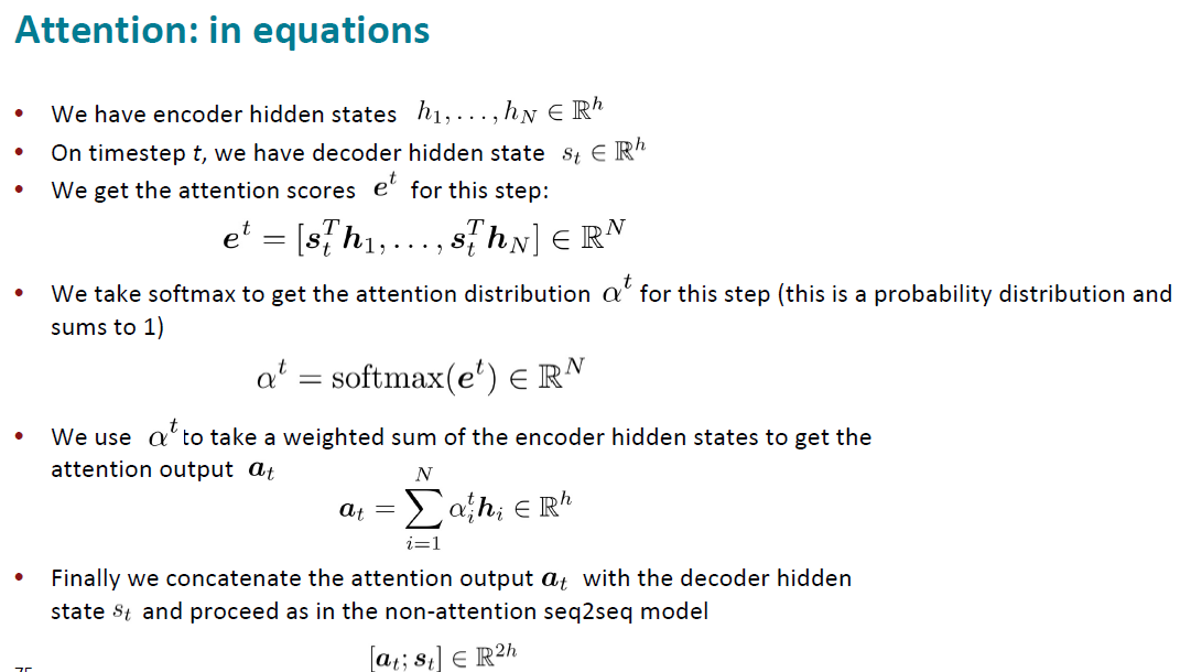
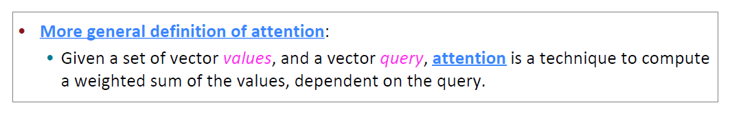
我们有时候会说: query attends to the
values,例如在seq2seq2+attention的模型中,每一个decoder hidden
state就是query,attends to 所有的encoder hidden states(values).
Attention is all you need
2017
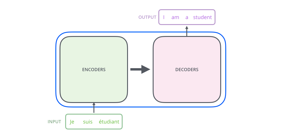
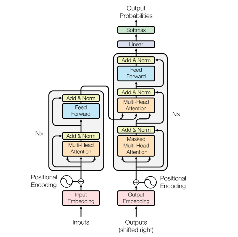
在transformer的paper中,作者首先介绍本文:主流的sequence
tranduction模型主要基于复杂的RNN或者CNN模型,它们包含encoder和decoder两部分,其中表现最好的模型在encoder和decoder之间增加了attention
mechanism。本文提出了一个新的简单的网络结构名叫transformer,也是完全基于attention机制,"dispensing
with recurrence and convolutions entirely"!
根本无需循环和卷积!了不起的Network~
在阅读这篇文章之前需要提前了解我在另外一篇博客 Attention and
transformer
model中的知识,在translation领域我们的科学家们是如何从RNN循环神经网络过渡到CNN,然后最终是transformer的天下的状态。技术经过了一轮轮的迭代,每一种基础模型架构提出后,会不断的有文章提出新的改进,文章千千万,不可能全部读完,就精读一些经典文章就好,Vaswani这篇文章是NMT领域必读paper,文章不长,加上参考文献才12页,介绍部分非常简单,导致这篇文章的入门门槛很高(个人感觉)。我一开始先读的这篇文章,发现啃不下去,又去找了很多资料来看,其中对我非常帮助的有很多:
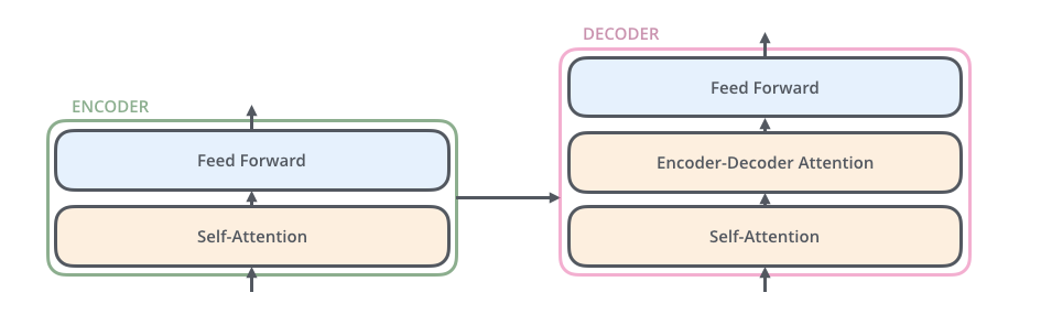
其中decoder部分的block比encoder部分的block多了一个sub
layer,其中self-attention和encoder-decoder attention都是multi-head
attention layer,只不过decoder部分的第一个multi-head attention
layer是一个masked multi-head
attention,为了防止未来的信息泄露给当下(prevent positions from
attending to the future).
# Merge the multi-head back to the original shape out = tf.concat(tf.split(out, self.h, axis=0), axis=2) # [bs, q_size, d_model]
# The final linear layer and dropout. # out = tf.layers.dense(out, self.d_model) # out = tf.layers.dropout(out, rate=self.drop_rate, training=self._is_training)
return out deffeed_forwad(self, inp, scope='ff'): """ Position-wise fully connected feed-forward network, applied to each position separately and identically. It can be implemented as (linear + ReLU + linear) or (conv1d + ReLU + conv1d). Args: inp (tf.tensor): shape [batch, length, d_model] """ out = inp with tf.variable_scope(scope): # out = tf.layers.dense(out, self.d_ff, activation=tf.nn.relu) # out = tf.layers.dropout(out, rate=self.drop_rate, training=self._is_training) # out = tf.layers.dense(out, self.d_model, activation=None)
# by default, use_bias=True out = tf.layers.conv1d(out, filters=self.d_ff, kernel_size=1, activation=tf.nn.relu) out = tf.layers.conv1d(out, filters=self.d_model, kernel_size=1)
return out defencoder_layer(self, inp, input_mask, scope): """ Args: inp: tf.tensor of shape (batch, seq_len, embed_size) input_mask: tf.tensor of shape (batch, seq_len, seq_len) """ out = inp with tf.variable_scope(scope): # One multi-head attention + one feed-forword out = self.layer_norm(out + self.multihead_attention(out, mask=input_mask)) out = self.layer_norm(out + self.feed_forwad(out)) return out
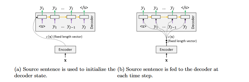
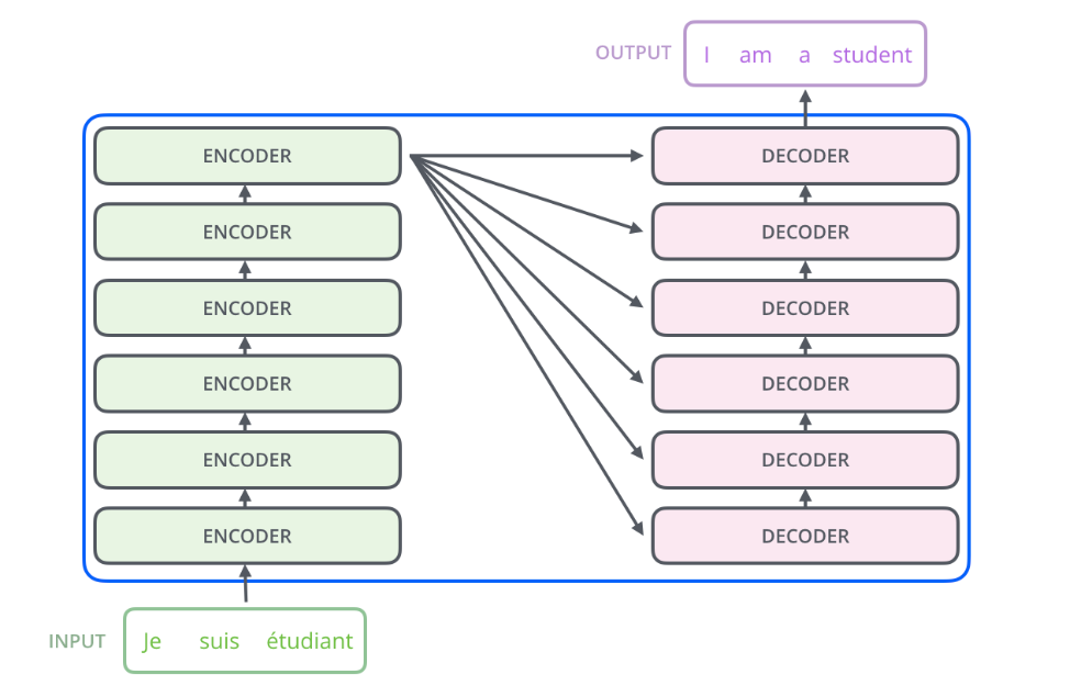
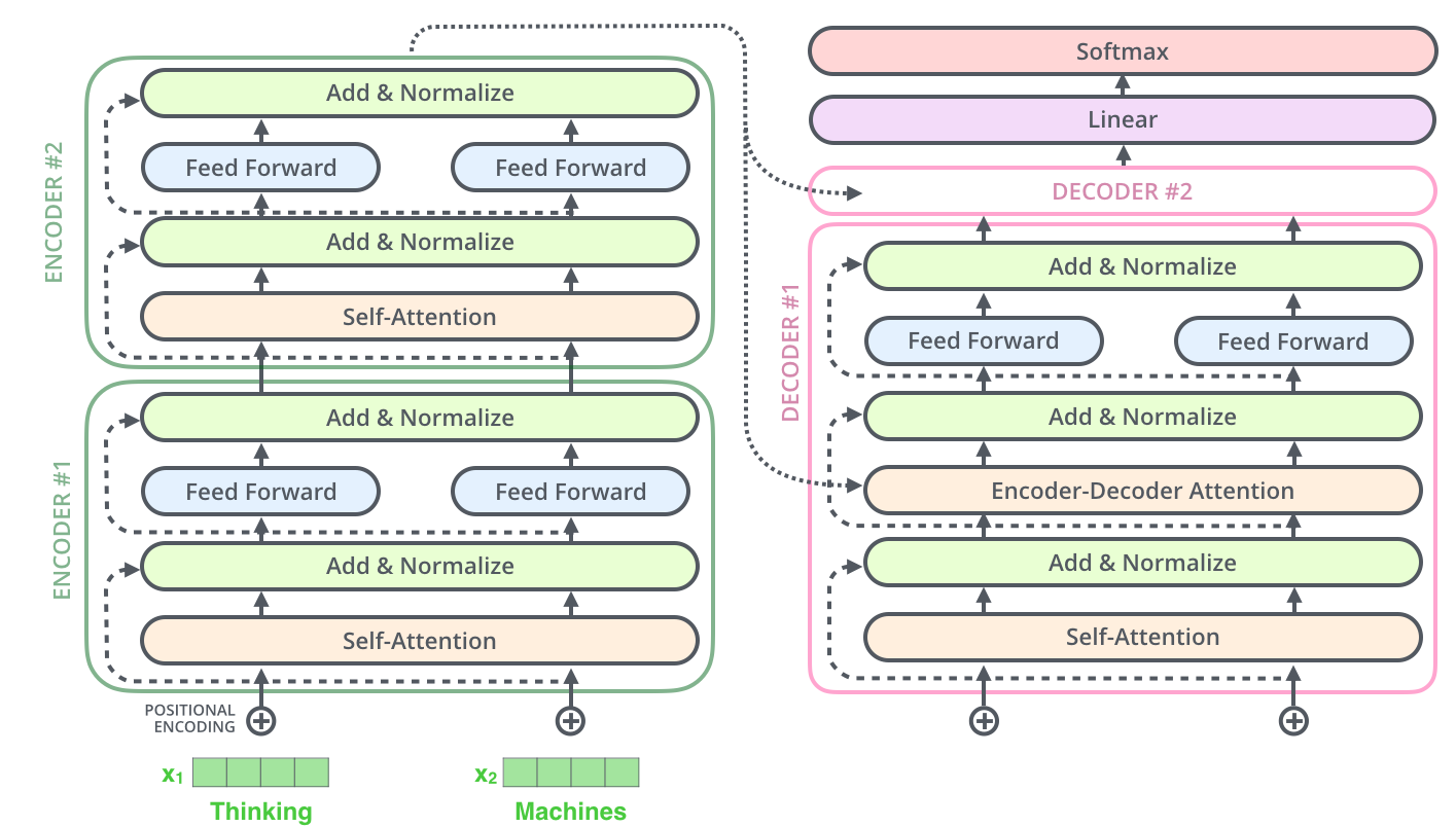
The encoder start by processing the input sequence. The output of the
top encoder is then transformed into a set of attention vectors K and V.
These are to be used by each decoder in its “encoder-decoder attention”
layer which helps the decoder focus on appropriate places in the input
sequence
defdecoder_layer(self, target, enc_out, input_mask, target_mask, scope): out = target with tf.variable_scope(scope): out = self.layer_norm(out + self.multihead_attention( out, mask=target_mask, scope='self_attn')) out = self.layer_norm(out + self.multihead_attention( out, memory=enc_out, mask=input_mask)) # 将encoder部分的输出结果作为输入 out = self.layer_norm(out + self.feed_forwad(out)) return out
defdecoder(self, target, enc_out, input_mask, target_mask, scope='decoder'): out = target with tf.variable_scope(scope): for i inrange(self.num_enc_layers): out = self.decoder_layer(out, enc_out, input_mask, target_mask, f'dec_{i}') return out
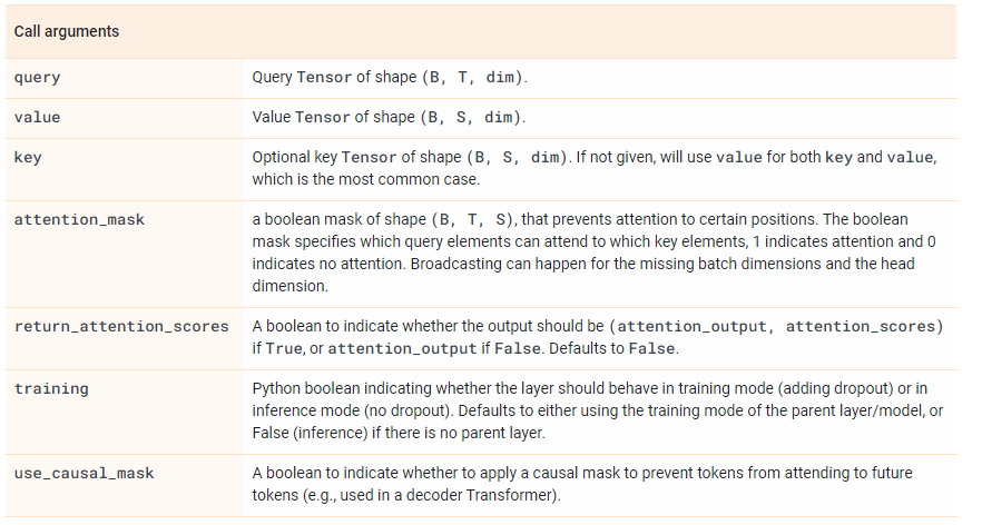
以上实现的transformer其实我觉得还是有一点点复杂,毕竟在tensorflow2.0+版本中已经有了官方实现好的layers.MultiHeadAttention可以使用,应该可以大大简化我们实现步骤,特别是上面的def multihead_attention(self, query, memory=None, mask=None, scope='attn'):。从刚刚的实现里我们可以发现,除了decoder部分每一个block的第二个sublayer的attention计算有一点不一样之外,其他的attention计算都是一模一样的。我在github上找了不少用TF2.0实现的transformer(最标准的也是Attention
is all you
need的模型),发现很多都都写得一般般,最终发现还是tensorflow官方文档写的tutotial写的最好.
classCausalSelfAttention(BaseAttention): defcall(self, x): attn_output = self.mha( query=x, value=x, key=x, use_causal_mask = True) # The causal mask ensures that each location only has access to the locations that come before it x = self.add([x, attn_output]) x = self.layernorm(x) return x
The Transformer (which will be referred to as
“vanilla Transformer” to distinguish it from other enhanced versions; Vaswani, et al., 2017) model
has an encoder-decoder architecture, as commonly used in many NMT
models. Later simplified Transformer was shown to achieve great
performance in language modeling tasks, like in encoder-only BERT
or decoder-only GPT.
# Block 1 x = tf.keras.layers.Conv2D(32, 3, strides=2, activation="relu")(input) x = tf.keras.layers.MaxPooling2D(3)(x) x = tf.keras.layers.BatchNormalization()(x)
# Block 2 x = tf.keras.layers.Conv2D(64, 3, activation="relu")(x) x = tf.keras.layers.BatchNormalization()(x) x = tf.keras.layers.Dropout(0.3)(x)
# Now that we apply global max pooling. gap = tf.keras.layers.GlobalMaxPooling2D()(x)
# Finally, we add a classification layer. output = tf.keras.layers.Dense(output_dim)(gap)
# bind all func_model = tf.keras.Model(input, output)
注意:这种方式最终要使用tf.keras.Model()来将inputs和outputs接起来。
Model sub-classing API 第三种方式是现在用的最多的方式。
之前我没理解layer和model两种调用方式的区别,我觉得就是一系列运算,我们把输入输进来,return
output结果的一个过程。但如果一个类它是Layer的子类,它比model的子类多了一个功能,它有state属性,也就是我们熟悉的weights。比如Dense
layer,我们知道它做了线性运算+激活函数,其中的weights就是我们assign给每一个feature的权重,但其实我们并不只是想要这一类别的运算,比如下面的:
def__init__(self, units=32, activation=None): '''Initializes the class and sets up the internal variables''' # YOUR CODE HERE super(SimpleQuadratic, self).__init__() self.units = units self.activation = tf.keras.activations.get(activation) defbuild(self, input_shape): '''Create the state of the layer (weights)''' # a and b should be initialized with random normal, c (or the bias) with zeros. # remember to set these as trainable. # YOUR CODE HERE a_init = tf.random_normal_initializer() b_init = tf.random_normal_initializer() c_init = tf.zeros_initializer() self.a = tf.Variable(name = "kernel", initial_value = a_init(shape= (input_shape[-1], self.units), dtype= "float32"), trainable = True) self.b = tf.Variable(name = "kernel", initial_value = b_init(shape= (input_shape[-1], self.units), dtype= "float32"), trainable = True) self.c = tf.Variable(name = "bias", initial_value = c_init(shape= (self.units,), dtype= "float32"), trainable = True) defcall(self, inputs): '''Defines the computation from inputs to outputs''' # YOUR CODE HERE result = tf.matmul(tf.math.square(inputs), self.a) + tf.matmul(inputs, self.b) + self.c return self.activation(result)
上面的代码将inputs平方之后和a做乘积,之后再加上inputs和b的乘积,最终返回的是和。这样的运算是tf.keras.layer中没有的。这个时候我们自己customize
layer就很方便。还有一个很方便的地方在于很多模型其实是按模块来的,模块内部的layer很类似。这个时候我们就可以把这些模型内的layer包起来变成一个layer的子类(Module),再定义完这些module之后我们使用Model把这些module再包起来,这就是我们最终的model。这时候我们就可以看到Model和Layer子类的区别了,虽然两者都可以实现输入进来之后实现一系列运算返回运算结果,但后者可以实现更灵活的运算,而前者往往是在把每一个模块定义好之后最终定义我们训练模型的类。
> In general, we use the Layer class to define the inner computation
blocks and will use the Model class to define the outer model,
practically the object that we will train. ---粘贴自博客
You can treat any model as if it were a layer by invoking it on an
Input or on the output of another layer. By calling a model
you aren't just reusing the architecture of the model, you're also
reusing its weights
defbuild_graph(self, raw_shape): x = tf.keras.layers.Input(shape=raw_shape) return Model(inputs=[x], outputs=self.call(x))
这样我们就可以正常调用summary()
1 2 3 4 5 6 7 8
cm.build_graph(raw_input).summary() # 不仅如此还能使用tf.keras.utils.plot_model来生成png tf.keras.utils.plot_model( model.build_graph(raw_input), # here is the trick (for now) to_file='model.png', dpi=96, # saving show_shapes=True, show_layer_names=True, # show shapes and layer name expand_nested=False# will show nested block )
@tf.function deftrain_step(step, x, y): ''' input: x, y <- typically batches input: step <- batch step return: loss value ''' # start the scope of gradient with tf.GradientTape() as tape: logits = model(x, training=True) # forward pass train_loss_value = loss_fn(y, logits) # compute loss
# update metrics train_acc_metric.update_state(y, logits) # write training loss and accuracy to the tensorboard with train_writer.as_default(): tf.summary.scalar('loss', train_loss_value, step=step) tf.summary.scalar( 'accuracy', train_acc_metric.result(), step=step ) return train_loss_value
先看如果一个函数不加这个装饰器会如何:
1 2 3 4 5 6 7
deff(x): print("Traced with", x)
for i inrange(5): f(2) f(3)
输出为:
1 2 3 4 5 6
Traced with 2 Traced with 2 Traced with 2 Traced with 2 Traced with 2 Traced with 3
加上装饰器:
1 2 3 4 5 6 7 8
@tf.function deff(x): print("Traced with", x)
for i inrange(5): f(2) f(3)
输出为:
1 2
Traced with2 Traced with3
可以看到第二种加了装饰器的方式,即便是循环了5遍,我们仍然只有一行打印了2.
如果我们在上面的代码中print之前加上一行:
1
2
3
4
5
6
7
8
9
@tf.function deff(x): print("Traced with", x) # add tf.print tf.print("Executed with", x) for i inrange(5): f(2) f(3)